Theoretical QM Rates vs. Experimental Heuristic Rates
KIMMDY can be used to sample competing reactions as long as proxies for comparable reaction rates are known. Let us consider the following two reactions that can occur in the backbone of a protein:
Homolysis of a bond
Hydrolysis of a bond
The KIMMDY-plugin version of earlier work on collagen bond rupture by Rennekamp et al. (2020) shipped with KIMMDY in the optional kimmdy-reactons package can be used to simulate force-dependent bond rupture reactions.
\[
k=A e^{-\Delta E / k_B T}
\tag{1}\]
Rennekamp et al. (2020) ultimately used an empirical attempt frequency of \(A=0.23 ps^{-1}\) (after starting with the theoretical maximal attempt frequency of \(A=6.25 ps^{-1}\)).
For hydrolysis, we take a a baseline energy barrier scaled by the force-dependence of the reaction unveiled by Pill et al. (2019). The observed attempt frequency of the hydrolysis reaction is further scaled by the solvent accessible surface area (SASA) of the peptide bond, normalized to the maximum SASA of a peptide bond in a lonely glycine-glycine dipeptide (\(=140 A^2\)).
Pill et al. (2019) suggest that the rate of the hydrolysis reaction is govered by two enegy barriers, where T1 is almost insensitive to mechanical activation, but only becomes rate-determining after the mechanically sensitive T2 is lowered by force.
TS1:
80 kJ/mol at 0nN
77 kJ/mol at 1.8nN
E = 80 - 1.67 * F
TS2:
92.5 kJ/mol at 0nN
46 kJ/mol at 1.8 nN
E = 92.5 - 25.83 * F
This translates to:
critical_force =0.7# nNif force < critical_force# low force regime, TS2 is rate-determining E_barrier =92.5-25.83* forceelse:# high force regime, TS1 is rate-determining E_barrier =80-1.67* force
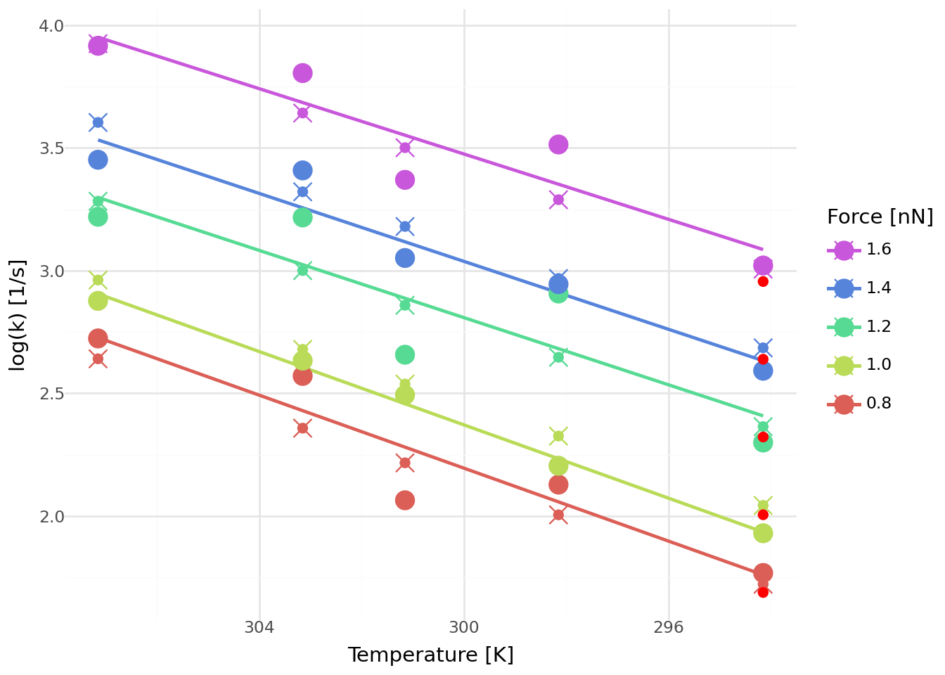
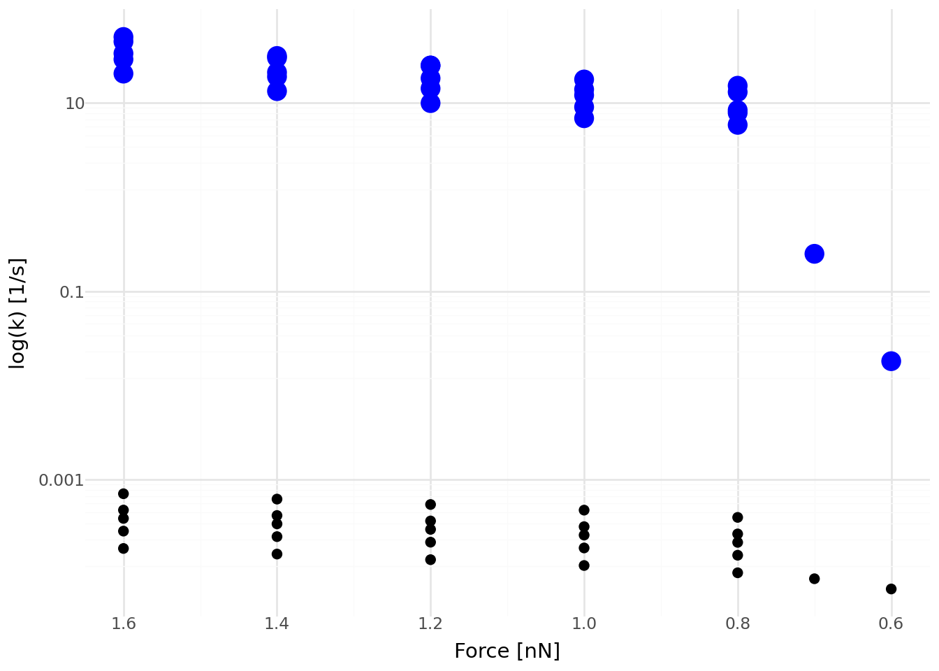
But the theortical rates don’t quite match the experimental rates.
from plotnine import*# pyright: ignoreimport matplotlib.pyplot as pltimport pandas as pdimport numpy as npfrom kimmdy_hydrolysis.rates import high_force_log_rate, theoretical_reaction_rate_per_s, experimental_reaction_rate_per_s, low_force_log_rateimport pandas as pdimport osroot = os.getcwd()theme_set(theme_minimal())
<plotnine.themes.theme_minimal.theme_minimal at 0x7782a2d13310>
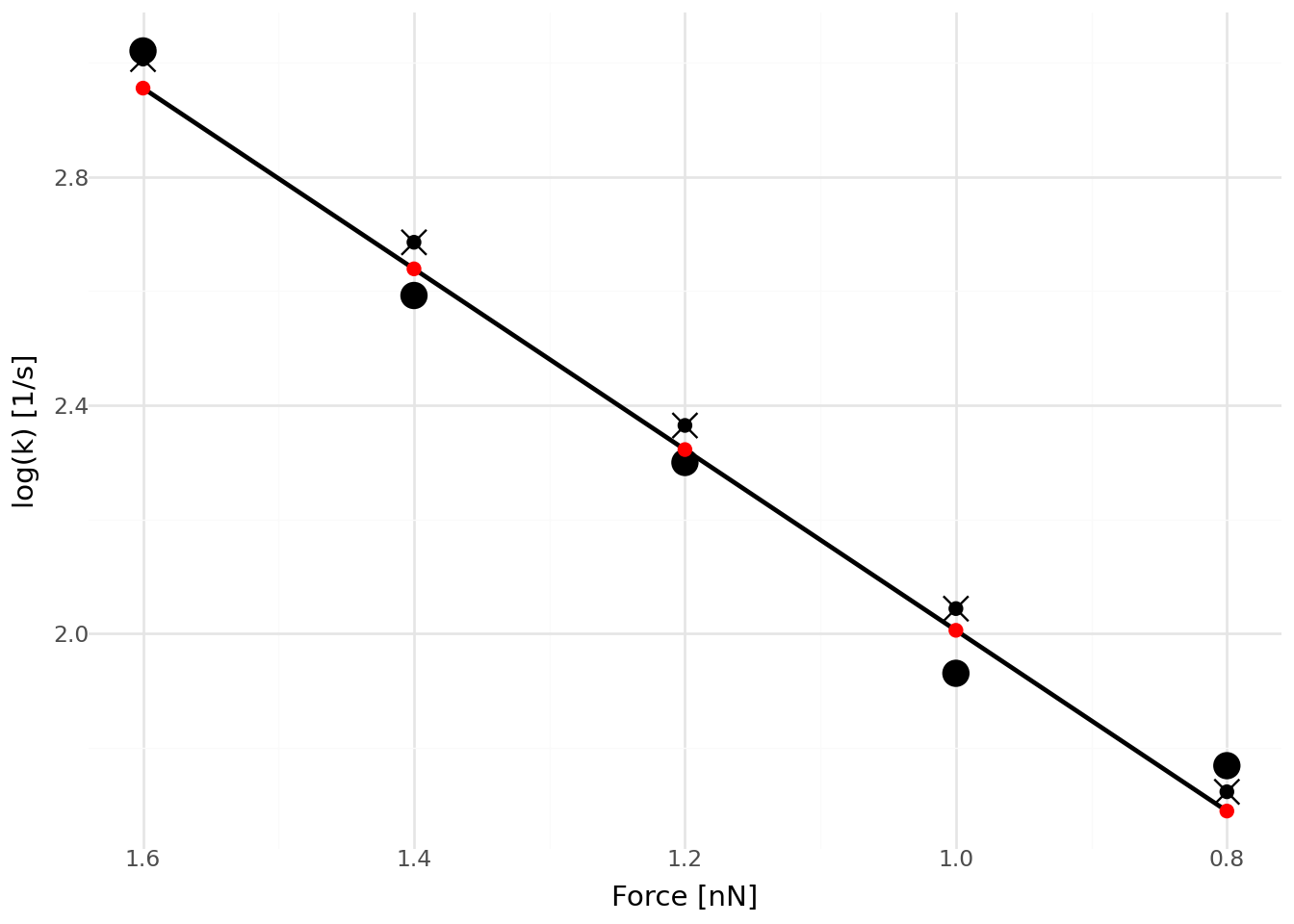
Instead of calculating rates from the theoretical energies we can fit the rates to the experimental data directly.
Get the data from the SI and add predicted rates from hydrolysis plugin function:
df = pd.read_csv("./assets/afm-rates.csv")df = df.melt(id_vars=["f"], var_name="t", value_name="rate")df["t"] = pd.to_numeric(df["t"], errors="coerce")df = df.dropna(subset=["rate"])df["log_k"] = np.log(df["rate"])df["is_low_f"] = df["f"] <=0.7df['plugin_k'] = [experimental_reaction_rate_per_s(force=f, temperature=t) for f, t inzip(df["f"], df["t"])]df['plugin_theo_k'] = [theoretical_reaction_rate_per_s(force=f, temperature=t) for f, t inzip(df["f"], df["t"])]df['plugin_high_log_k'] = [high_force_log_rate(force=f, temperature=t) for f, t inzip(df["f"], df["t"])]df['plugin_low_log_k'] = [low_force_log_rate(force=f) for f, t inzip(df["f"], df["t"])]df['plugin_log_k'] = np.log(df['plugin_k'])
Fit model log(k) ~ t + f:
import statsmodels.api as smmodel = sm.OLS.from_formula("log_k ~ t + f", data=df.query("not is_low_f"))model.fit().summary()
OLS Regression Results
Dep. Variable:
log_k
R-squared:
0.944
Model:
OLS
Adj. R-squared:
0.939
Method:
Least Squares
F-statistic:
187.0
Date:
Thu, 12 Jun 2025
Prob (F-statistic):
1.56e-14
Time:
14:32:26
Log-Likelihood:
14.858
No. Observations:
25
AIC:
-23.72
Df Residuals:
22
BIC:
-20.06
Df Model:
2
Covariance Type:
nonrobust
coef
std err
t
P>|t|
[0.025
0.975]
Intercept
-20.3430
1.946
-10.453
0.000
-24.379
-16.307
t
0.0706
0.006
10.940
0.000
0.057
0.084
f
1.6052
0.101
15.946
0.000
1.396
1.814
Omnibus:
3.044
Durbin-Watson:
2.069
Prob(Omnibus):
0.218
Jarque-Bera (JB):
2.094
Skew:
0.523
Prob(JB):
0.351
Kurtosis:
2.044
Cond. No.
2.06e+04
Notes: [1] Standard Errors assume that the covariance matrix of the errors is correctly specified. [2] The condition number is large, 2.06e+04. This might indicate that there are strong multicollinearity or other numerical problems.
Pill, Michael F., Allan L. L. East, Dominik Marx, Martin K. Beyer, and Hauke Clausen-Schaumann. 2019. “Mechanical Activation Drastically Accelerates Amide Bond Hydrolysis, Matching Enzyme Activity.”https://doi.org/10.1002/anie.201902752.
Rennekamp, Benedikt, Fabian Kutzki, Agnieszka Obarska-Kosinska, Christopher Zapp, and Frauke Gräter. 2020. “Hybrid Kinetic Monte Carlo/Molecular Dynamics Simulations of Bond Scissions in Proteins.”https://doi.org/10.1021/acs.jctc.9b00786.