SITH Analysis Tutorial
In this tutorial, you will learn how to analyse the outcome of your
stretching simulations with sith. You will obtain the distribution of
energies in a Glycine amino acid with NME and ACE capping groups pulled
at the ends (Figure 1). From the outset, we assume that you have a
directory containing fchk files in sith format with the QM
information, and that you are running the Python scripts from this
tutorial in the same directory. If you do not yet have these files, you
can download them from
https://github.com/Sucerquia/Gdata4tut, or check the
Stretching Molecule Tutorial if you wish to generate them yourself.
The first step is to load the data into a sith.SITH.SITH object:
1from sith import SITH
2
3sith = SITH('./forces')
4# The next line could also be jedi_analysis if your fchk files
5# contain the Hessian matrix of the optimised configuration.
6sith.sith_analysis();
Visualising the Stretching of your Molecule
Note
sith has an integrated visualisation tool, which requires that you first install VPython and VMol. You may skip this part of the tutorial if preferred.
As a simpler alternative to observe the stretching, you can use, for example,
vmd *.xyz.
First, check the trajectory collected by sith.SITH.SITH. This
is taken from the fchk files in your directory, sorted alphabetically.
If your trajectory appears disordered, rename the files in increasing order.
1from sith.visualize.vmol import EnergiesVMol as Evmol
2
3v = Evmol(sith, absolute=True, alignment=[1, 16, 13],
4          height=300, default_bonds=True)
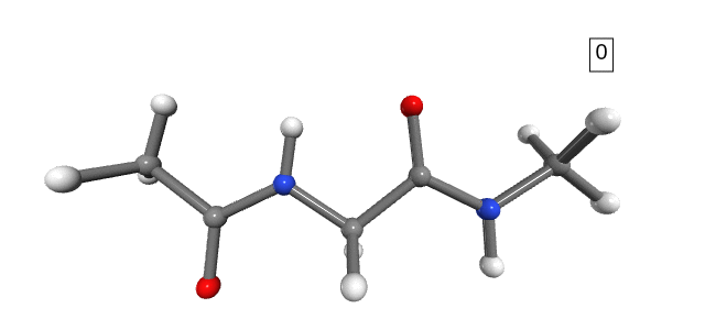
Figure 1. Stretching path. The number shown in the box is the stretching state.
Notice that the dihedral angles of the hydrogens in the NME capping group change drastically between stretching 1 and stretching 2 (Figure 1). However, we do not expect any significant energy distribution in the degrees of freedom of the hydrogens, as they are too light and not part of the connecting bonds (only side-chains). For the purpose of analysis, and to avoid numerical errors caused by the large changes in the hydrogens’ degrees of freedom, we can simply exclude them from the calculation.
1sith = SITH('./forces')
2sith.killer(killElements='H')
3sith.sith_analysis();
You can then visualise the evolution of the distribution of energies in the interatomic distances (Figure 2).
 1# The next two lines define the colourmap used in this tutorial.
 2# You may use any other colormap you prefer, for example,
 3# matplotlib.colormaps['Blues']
 4import cmocean as cmo
 5
 6cmap = cmo.cm.algae
 7
 8v = Evmol(sith, dofs=['bonds'], cmap=cmap, absolute=True, deci=4,
 9          labelsize=5, alignment=[1, 16, 13])
10v.update_stretching(8)
11v.add_image_to_canvas(v.fig);
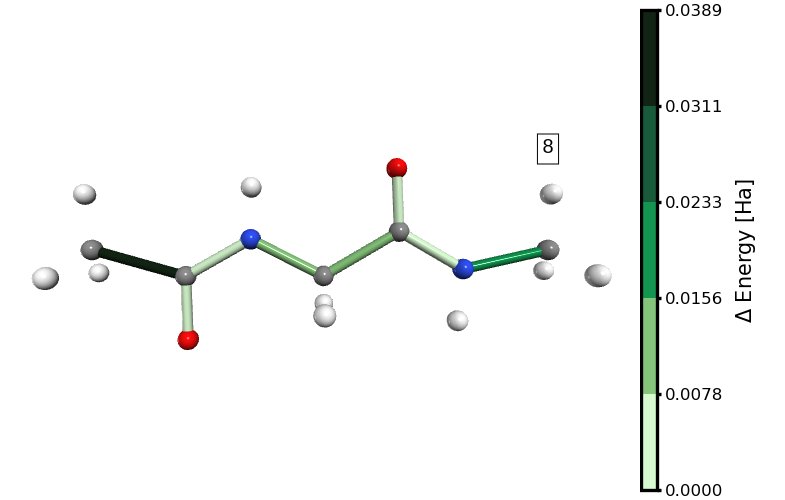
Figure 2. Energy distribution in distances at the 8th stretching step (immediately before the rupture of the molecule). The links to the hydrogen atoms are not shown because we excluded them from the analysis.
In Figure 2, it is clear that at the 8th stretching state the bond energy is concentrated mainly in the C\(\alpha\)-C bond of the ACE capping group, followed by the C-N bond of the NME capping group. This is, of course, only a visual inspection. In the next section, we will perform a more quantitative analysis of this energy distribution.
In the same way, you could visualise the distribution of energies only in the angles or in the dihedrals. Alternatively, you could include a comparison considering both angles and bonds (Figure 3).
1v = Evmol(sith, dofs=['angles', 'bonds'], cmap=cmap, absolute=True, deci=4,
2          alignment=[1, 16, 13], labelsize=5, default_bonds=True)
3v.update_stretching(8)
4v.add_image_to_canvas(v.fig);
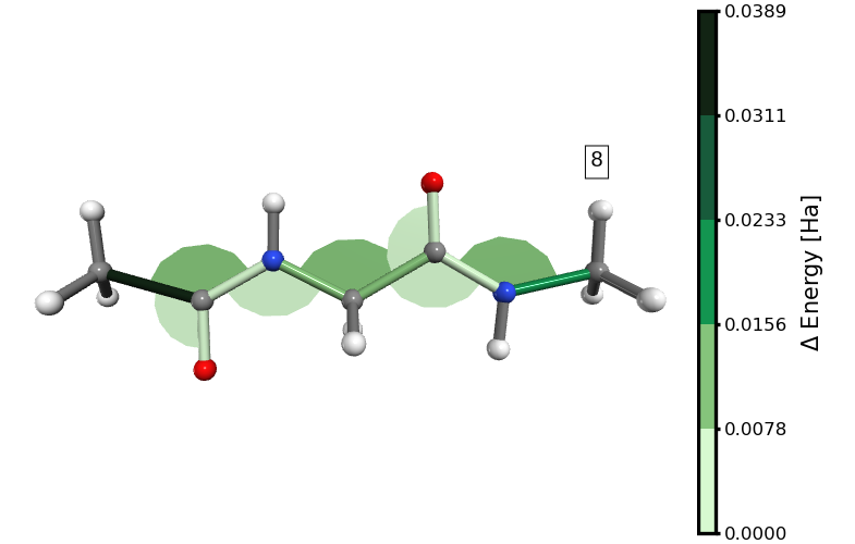
Figure 3. Energy distribution in distances and angles at the 8th stretching step (immediately before the rupture of the molecule). The links to the hydrogen atoms are grey because we excluded them from the analysis, but they have been added as “default_bonds” for illustrative purposes.
We can immediately observe that the energy is mostly stored in the bonds, even when the energy associated with some angles is higher than that of certain bonds.
Note
The visualisation of dihedrals may fail because of an internal error in VPython. The error message you may see is:
TypeError: unsupported operand type(s) for *: 'float' and 'vpython.cyvector.vector'.
Quantitative Analysis
Getting to Know SITH Attributes
With the following Python commands, you can inspect the values stored
in the sith.SITH.SITH object.
1import inspect
2
3[print(name) for name, value in inspect.getmembers(sith)
4 if not callable(value) and not name.startswith("__")];
all_dofs
all_forces
delta_q
dim_indices
dims
dofs_energies
energies_percentage
n_structures
reference
removed_dofs
structure_energies
structures
structures_scf_energies
The names of the most important values are largely
self-explanatory (remember that dofs stands for Degrees of Freedom).
For further details on these attributes, see sith.SITH.SITH.
Here, we briefly discuss how they help in analysing the distribution of
energies.
In sith, all quantities that depend on the stretching and the
degrees of freedom are stored as NumPy arrays, where axes 0 and 1
correspond to the stretching state and the degrees of freedom,
respectively. The stretching state increases monotonically, while the
index order of the degrees of freedom is defined in
sith.SITH.SITH.dim_indices.
Note also that sith.SITH.SITH.dims has four components,
corresponding to the total number of Degrees of Freedom, the number of
distances, the number of angles, and the number of dihedrals, in that
order.
SITH Analysis
In this section, we plot some of the key quantities in sith and
briefly comment on them.
Note
We are using PlottingTool together with Matplotlib, but you are free to use any plotting tool you prefer. The important lines are highlighted; the rest are simply visualisation settings.
Internal Forces
In the following Python script, we plot the forces in the different
degrees of freedom (distances, angles, and dihedrals). The relevant
attribute here is sith.SITH.SITH.all_forces.
We plot all the forces across all stretching states (the : slice
selects all entries along axis 0 of all_forces). We then extract the
subsets corresponding to distances, angles, and dihedrals. Each curve
represents the force evolution across stretching states for a given
degree of freedom, labelled by its DOF index.
 1from PlottingTool import StandardPlotter
 2import numpy as np
 3import matplotlib.pyplot as plt
 4
 5fig, axes = plt.subplots(3, 1)
 6sp = StandardPlotter(fig=fig, figheight=14,
 7                     ax=axes, ax_pref={'xticks': range(0, 9)})
 8
 9sp.plot_data(range(0, 9),
10             sith.all_forces[:, :sith.dims[1]].T,
11             ax=0, ms=2, lw=1,
12             data_label=np.arange(sith.dims[1]))
13sp.plot_data(range(0, 9),
14             sith.all_forces[:, sith.dims[1]: sith.dims[1] + sith.dims[2]].T,
15             data_label=np.arange(sith.dims[1], sith.dims[1] + sith.dims[2]),
16             ax=1, ms=2, lw=1)
17sp.plot_data(range(0, 9),
18             sith.all_forces[:, -sith.dims[3]:].T,
19             data_label=np.arange(sith.dims[0] - sith.dims[3], sith.dims[0]),
20             ax=2, ms=2, lw=1)
21
22sp.axis_setter(ax=0, xticks=[], xminor=range(0, 9), legend=True,
23               ylabel='F in Distance\n[Ha/Å]')
24sp.axis_setter(ax=1, xticks=[], xminor=range(0, 9), legend=True,
25               ylabel='F in Angle\n[Ha/rad]')
26sp.axis_setter(ax=2, legend=True, xlabel='Stretched Configuration',
27               ylabel='F in Dihedral\n[Ha/rad]')
28
29sp.spaces[0].set_axis(rows_cols=(3, 1), borders=[[0.16, 0.065], [0.99, 0.97]],
30                      spaces=(0.1, 0.05));
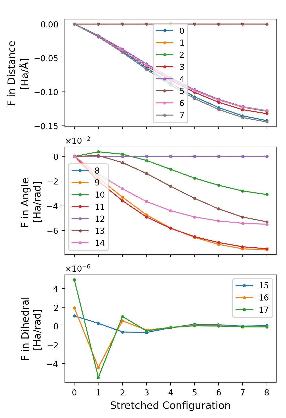
Figure 4. Forces per stretched structure for each degree of freedom,
separated into distances, angles, and dihedrals. The labels correspond to
the indices of the DOFs in sith.
Changes in the Degrees of Freedom
Another important attribute of sith is the change in the values of the
degrees of freedom (sith.SITH.SITH.delta_q), which in this case
is defined by
sith.energy_analysis.sith_analysis.SithAnalysis.get_sith_dq(). This is
a crucial quantity (along with the forces) because, for numerical
integration, the steps must be sufficiently small to ensure a reasonable
discretisation of the energy integral. In this example, all changes in
distances are below 0.1 Å, while the angular changes remain under 4°.
 1fig, axes = plt.subplots(3, 1)
 2sp = StandardPlotter(fig=fig, ax=axes, figheight=14)
 3
 4sp.plot_data(range(0, 9),
 5             sith.delta_q[:, :sith.dims[1]].T,
 6             data_label=np.arange(sith.dims[1]),
 7             ax=0, ms=2, lw=1)
 8sp.plot_data(range(0, 9),
 9             sith.delta_q[:, sith.dims[1]: sith.dims[1] + sith.dims[2]].T * 180 / 3.14159,
10             data_label=np.arange(sith.dims[1], sith.dims[1] + sith.dims[2]),
11             ax=1, ms=2, lw=1)
12sp.plot_data(range(0, 9),
13             sith.delta_q[:, -sith.dims[3]:].T * 180 / 3.14159,
14             data_label=np.arange(sith.dims[0] - sith.dims[3], sith.dims[0]),
15             ax=2, ms=2, lw=1)
16
17sp.axis_setter(ax=0, xticks=[], xminor=range(0, 9), legend=True,
18               ylabel='$\Delta$ Distances [Å]')
19sp.axis_setter(ax=1, xticks=[], xminor=range(0, 9), legend=True,
20               ylabel='$\Delta$ Angles [°]')
21sp.axis_setter(ax=2, xminor=range(0, 9), legend=True, xlabel='Stretched Configuration',
22               ylabel='$\Delta$ Dihedrals [°]')
23
24sp.spaces[0].set_axis(rows_cols=(3, 1), borders=[[0.16, 0.1], [0.99, 0.99]],
25                      spaces=(0.1, 0.05));
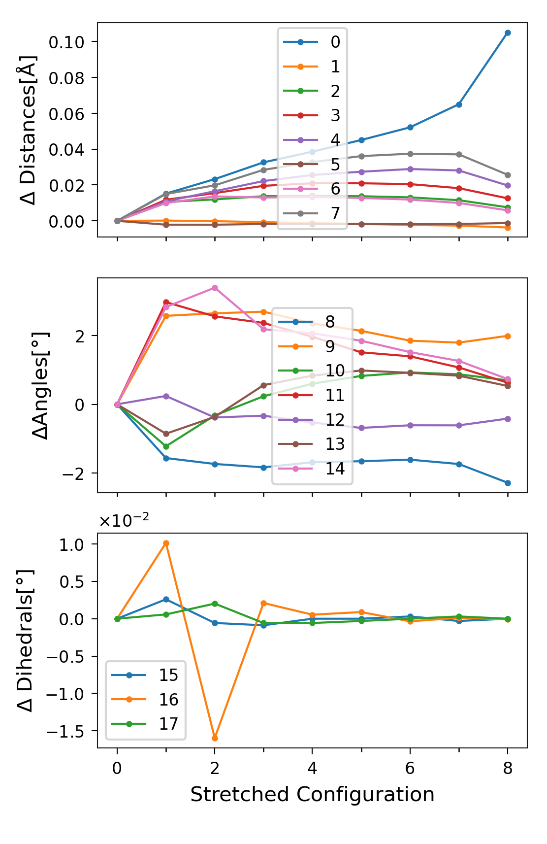
Figure 5. \(\Delta q_i\) per stretched structure for each degree of
freedom, separated into distances, angles, and dihedrals
(\(q_i\) denotes the value of the i-th` degree of freedom).
Labels correspond to the DOF indices in sith.
Values of the DOFs
Instead of plotting only the changes, we can plot the actual values of
the degrees of freedom at each stretching state. These are stored in
sith.SITH.SITH.all_dofs.
 1fig, axes = plt.subplots(3, 1)
 2sp = StandardPlotter(fig=fig, ax=axes, figheight=14)
 3
 4sp.plot_data(range(0, 9),
 5             sith.all_dofs[:, :sith.dims[1]].T,
 6             data_label=np.arange(sith.dims[1]),
 7             ax=0, ms=2, lw=1)
 8sp.plot_data(range(0, 9),
 9             sith.all_dofs[:, sith.dims[1]: sith.dims[1] + sith.dims[2]].T * 180 / 3.14159,
10             data_label=np.arange(sith.dims[1], sith.dims[1] + sith.dims[2]),
11             ax=1, ms=2, lw=1)
12sp.plot_data(range(0, 9),
13             sith.all_dofs[:, -sith.dims[3]:].T * 180 / 3.14159,
14             data_label=np.arange(sith.dims[0] - sith.dims[3], sith.dims[0]),
15             ax=2, ms=2, lw=1)
16
17sp.axis_setter(ax=0, xticks=[], xminor=range(0, 9), legend=True,
18               ylabel='Distances [Å]')
19sp.axis_setter(ax=1, xticks=[], xminor=range(0, 9), legend=True,
20               ylabel='Angles [°]')
21sp.axis_setter(ax=2, xminor=range(0, 9), legend=True, xlabel='Stretched Configuration',
22               ylabel='Dihedrals [°]')
23
24sp.spaces[0].set_axis(rows_cols=(3, 1), borders=[[0.16, 0.1], [0.99, 0.99]],
25                      spaces=(0.1, 0.05));
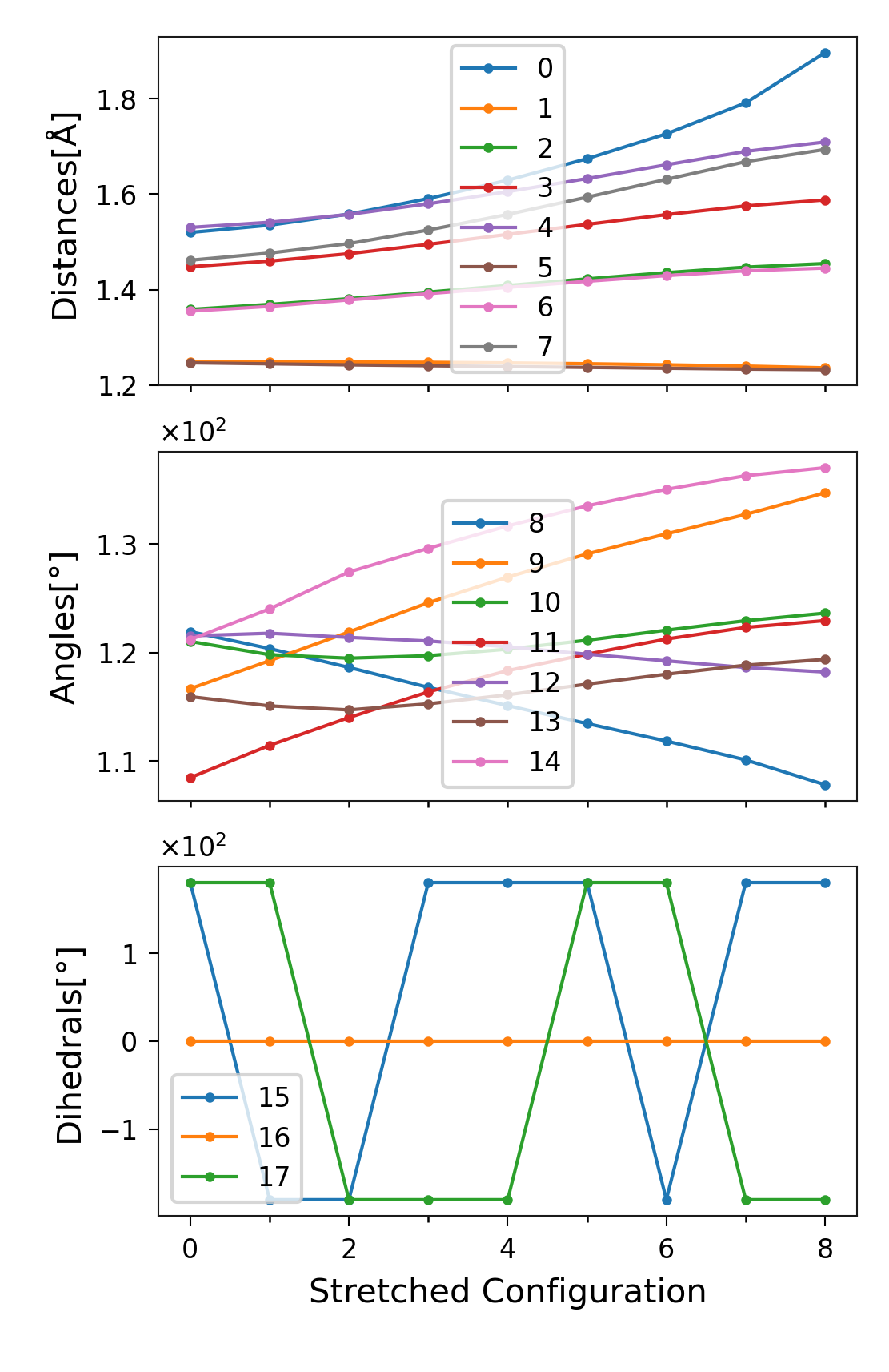
Figure 6. \(q_i\) per stretched structure for each degree of
freedom, separated into distances, angles, and dihedrals
(\(q_i\) denotes the value of the i-th degree of freedom).
Labels correspond to the DOF indices in sith.
In the plot of dihedral changes (Figure 5 lowest plot), there did not appear to be any large variation. However, in this plot the dihedrals seem to exhibit large jumps. These jumps are in fact artefacts of visualisation, caused by the periodicity of the angles (181\(^\circ\) = -179\(^\circ\)). As we present in the last section of this tutorial, polar plots are better to visualise this kind of data.
The Distribution of Energies
The principal aim of sith is to compute the distribution of energies.
This quantity is stored in sith.SITH.SITH.dofs_energies.
 1fig, axes = plt.subplots(3, 1)
 2sp = StandardPlotter(fig=fig, ax=axes, figheight=16)
 3
 4sp.plot_data(np.cumsum(sith.delta_q[:, :sith.dims[1]].T, axis=1),
 5             sith.dofs_energies[:, :sith.dims[1]].T,
 6             ax=0, ms=2, lw=1, data_label=np.arange(sith.dims[1]))
 7sp.plot_data(np.cumsum(sith.delta_q[:, sith.dims[1]: sith.dims[1] + sith.dims[2]].T * 180 / 3.14159,
 8                       axis=1),
 9             sith.dofs_energies[:, sith.dims[1]: sith.dims[1] + sith.dims[2]].T,
10             data_label=np.arange(sith.dims[1], sith.dims[1] + sith.dims[2]),
11             ax=1, ms=2, lw=1)
12sp.plot_data(np.cumsum(sith.delta_q[:, -sith.dims[3]:].T * 180 / 3.14159, axis=1),
13             sith.dofs_energies[:, -sith.dims[3]:].T,
14             data_label=np.arange(sith.dims[0] - sith.dims[3], sith.dims[0]),
15             ax=2, ms=2, lw=1)
16
17sp.axis_setter(ax=0,
18               xlabel='$\Delta$ Distance [Å]',
19               ylabel='$\Delta$ Energy [Ha]',
20               legend=True)
21sp.axis_setter(ax=1,
22               xlabel='$\Delta$ Angles [°]',
23               ylabel='$\Delta$ Energy [Ha]',
24               legend=True)
25sp.axis_setter(ax=2,
26               xlabel='$\Delta$ Dihedrals [°]',
27               ylabel='$\Delta$ Energy [Ha]',
28               xticks=[-0.005, 0, 0.005, 0.01],
29               legend=True)
30
31sp.spaces[0].set_axis(rows_cols=(3, 1), borders=[[0.16, 0.065], [0.99, 0.97]],
32                      spaces=(0.1, 0.1));
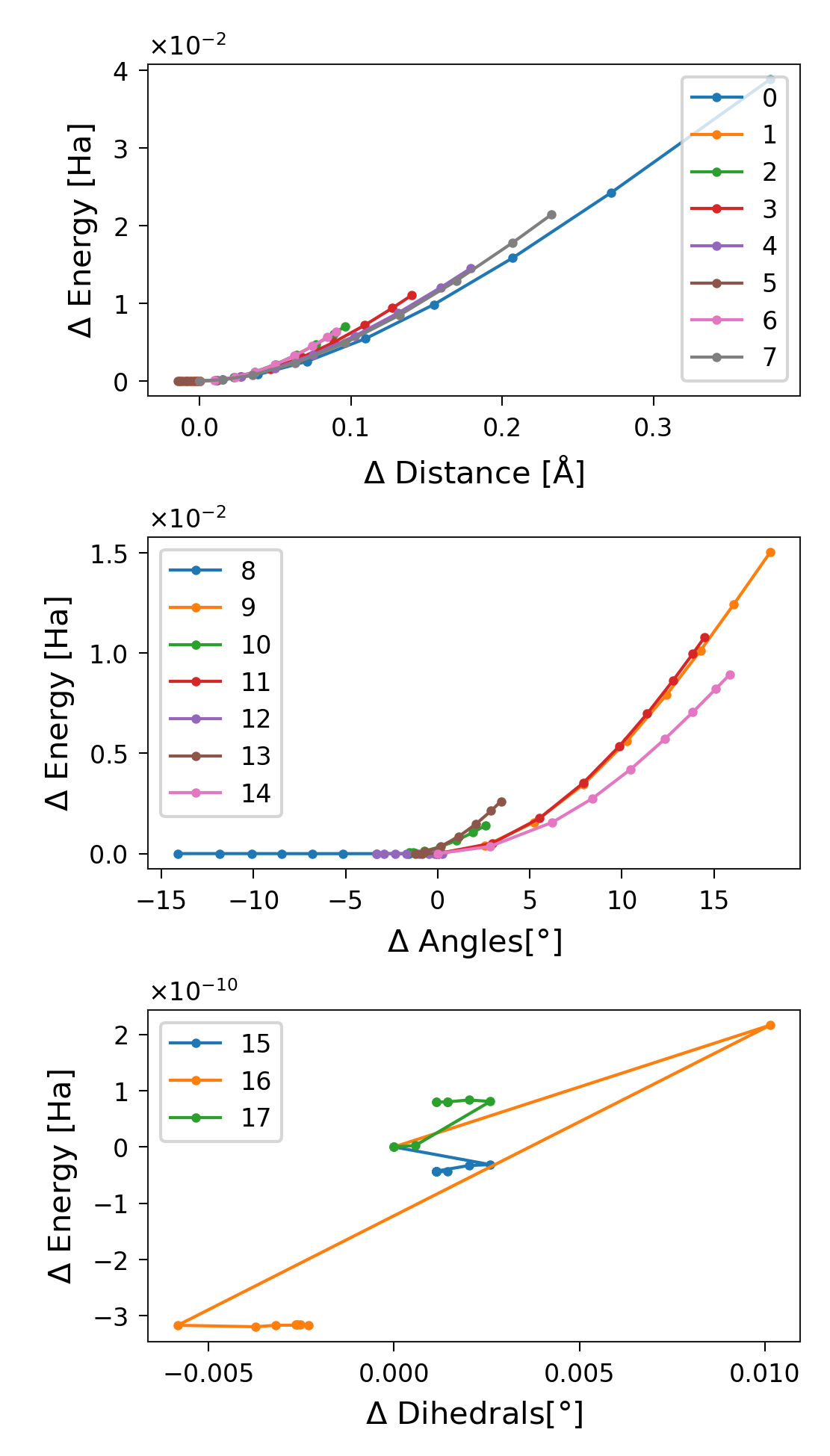
Figure 7. Energy distribution per stretched structure for each degree of
freedom, separated into distances, angles, and dihedrals. Labels correspond
to the DOF indices in sith.
Note that the degree of freedom with index 5 (C-O distance in Glycine) does not store any energy; its value even decreases slightly. The same is true for DOF index 8 (C-O-C angle of the ACE capping group). This behaviour is perfectly normal and reflects the relaxation of the molecule during stretching. A change in a degree of freedom does not necessarily imply that it stores energy; there must also be a non-zero force associated with it. In other words, the external force modifies the potential energy surface such that the equilibrium position of that degree of freedom shifts, while its energy remains unchanged.
Another important observation is that the energy stored in the dihedrals appears chaotic. This results from numerical noise at very small magnitudes, which appear random. Compare this with the plots of dihedral changes and forces shown earlier (Figures 4 and 5).
Finally, we see that the energy stored in the degrees of freedom always increases rather than decreases. This makes perfect sense, since we begin at a minimum-energy configuration, from which the energy can only increase.
Energy in a Specific DOF
Suppose you want the energy stored specifically in the distance between
atoms 9 and 12 (using the 1-based convention). First, locate this DOF in
sith.SITH.SITH.dim_indices. Once you find it, note its index
(4 in this case), and use it to plot the corresponding energy:
1sp = StandardPlotter()
2sp.plot_data(np.cumsum(sith.delta_q[:, 4]),
3             sith.dofs_energies[:, 4],
4             data_label='9-12 distance', ms=2, lw=1);
5sp.axis_setter(xticks=[0, 0.05, 0.1, 0.15], xlabel='$\Delta$ Distance [Å]',
6               ylabel='$\Delta$ Energy [Ha]', legend=True)
7
8sp.spaces[0].set_axis(borders=[[0.145, 0.14], [0.99, 0.95]]);
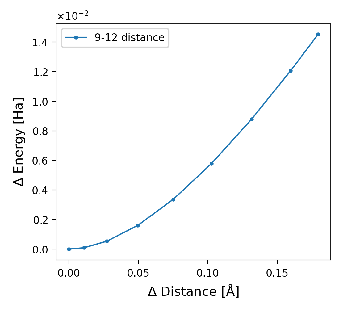
Figure 8. Energy stored in the degree of freedom with index 4, corresponding to the distance between atoms 9 and 12.
SithPlotter
sith includes a tool for data visualisation that proves useful for
analysis, particularly when focusing on a specific bond identifiable by
the atom names (see example below). The tool requires a PDB file containing
molecular information, such as residue numbers and atom names. We initially
developed it for amino acid analysis, but we are extending it to support
any type of molecule. For now, you can apply the tools demonstrated here by
treating “amino” as any residue in your PDB file.
1from sith.utils.sith_plots import SithPlotter
2
3pdb = './G.pdb'
4plotter_sith = SithPlotter(sith, pdb)
sith.utils.sith_plots provides two attributes: amino_name and
amino_info. amino_name stores the names of the residues, while
amino_info stores the atom names for each residue along with their
indices (1-based).
1print(plotter_sith.amino_name)
2print(plotter_sith.amino_info)
{1: 'ACE ', 2: 'GLY ', 3: 'NME '}
{1: {'CH3': 1, '1HH3': 2, '2HH3': 3, '3HH3': 4, 'C': 5, 'O': 6},
 2: {'N': 7, 'H': 8, 'CA': 9, 'HA1': 10, 'HA2': 11, 'C': 12, 'O': 13},
 3: {'N': 14, 'H': 15, 'CH3': 16, '1HH3': 17, '2HH3': 18, '3HH3': 19}}
To select the index of the \(C_\alpha\) and C atoms of Glycine (the second residue), run:
1print(plotter_sith.amino_info[2]['CA'], plotter_sith.amino_info[2]['C'])
9 12
To find the index corresponding to the distance separating these two atoms, run:
1plotter_sith.index_dof(np.array([9, 12, 0, 0]))
4
Energy in a DOF Defined by Atom Name
Once you identify the index, you can plot the energy in this specific
degree of freedom, as shown in Figure 8. Alternatively, use the method
sith.utils.sith_plots.SithPlotter.le_dof_amino().
1sp = StandardPlotter(ax_pref={'xlabel': r'C$\alpha$-C Length [Å]',
2                              'ylabel': r'E$_{C_\alpha-C}$ [Ha]',
3                              'xticks': [1.55, 1.6, 1.65, 1.7]})
4l, e = plotter_sith.le_dof_amino(('CA', 'C'), 2)
5sp.plot_data(l, e)
6sp.spaces[0].locate_ax(borders=[[0.14, 0.130], [0.99, 0.95]])
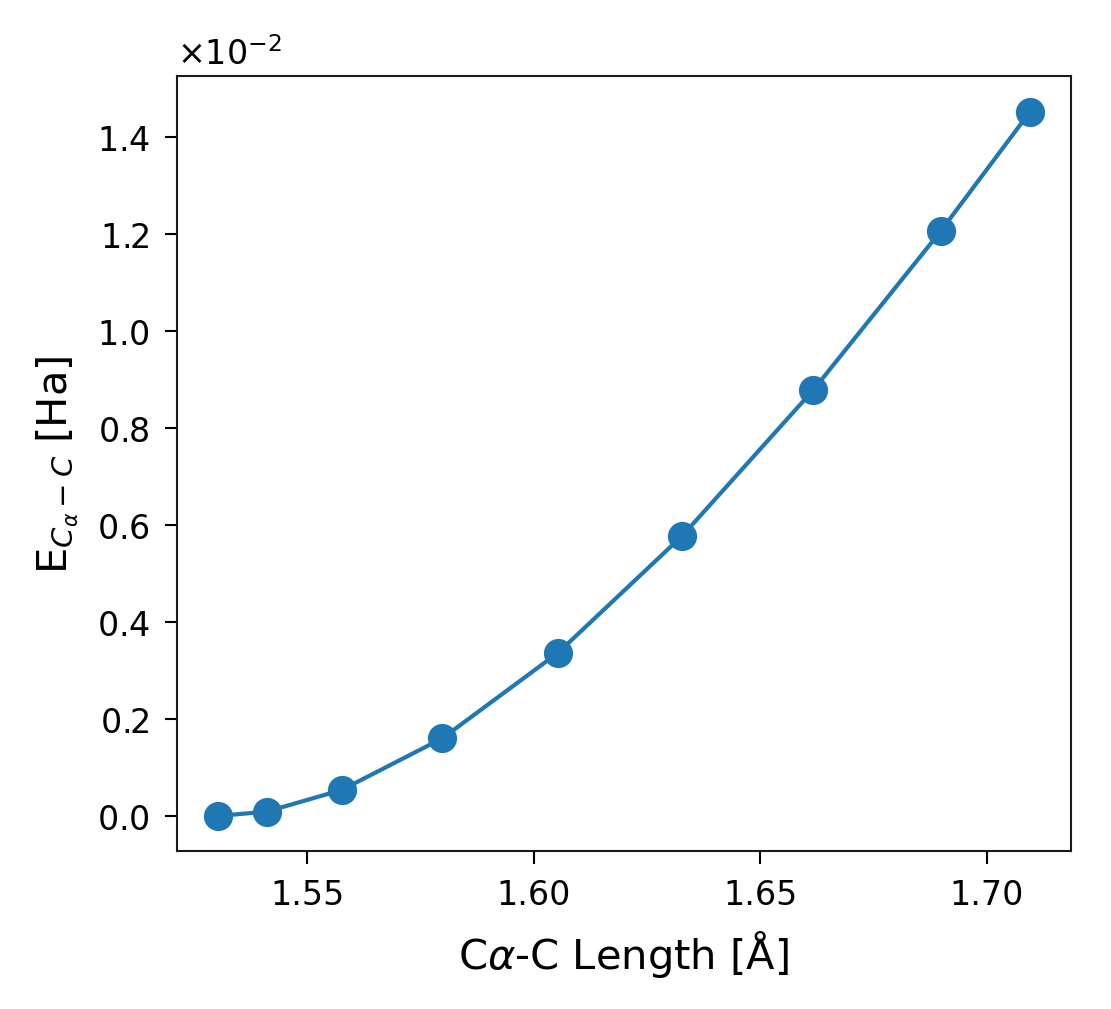
Figure 9. Energy stored in the degree of freedom corresponding to the distance between the C\(\alpha\) and C atoms of Glycine (second residue of the system).
Checking Harmonicity in a Single DOF
Methods such as JEDI (T. Stauch and A. Dreuw, 2016, Chem. Rev., 116) assume a harmonic approximation for energy distributions in each degree of freedom. sith allows you to examine how closely a specific degree of freedom follows a harmonic potential. For example, consider the C\(\alpha\)-C distance plotted above. If the distribution perfectly approximates a harmonic potential, the resulting plot forms a straight line.
1sp = StandardPlotter(ax_pref={'xlabel': r'C$\alpha$-C Length [Å]',
2                              'ylabel': r'$\sqrt{E_{C_\alpha-C}} [\sqrt{Ha}]$',
3                              'xticks': [1.55, 1.6, 1.65, 1.7]})
4sp.plot_data(l, np.sqrt(e))
5sp.spaces[0].locate_ax(borders=[[0.14, 0.130], [0.99, 0.95]])
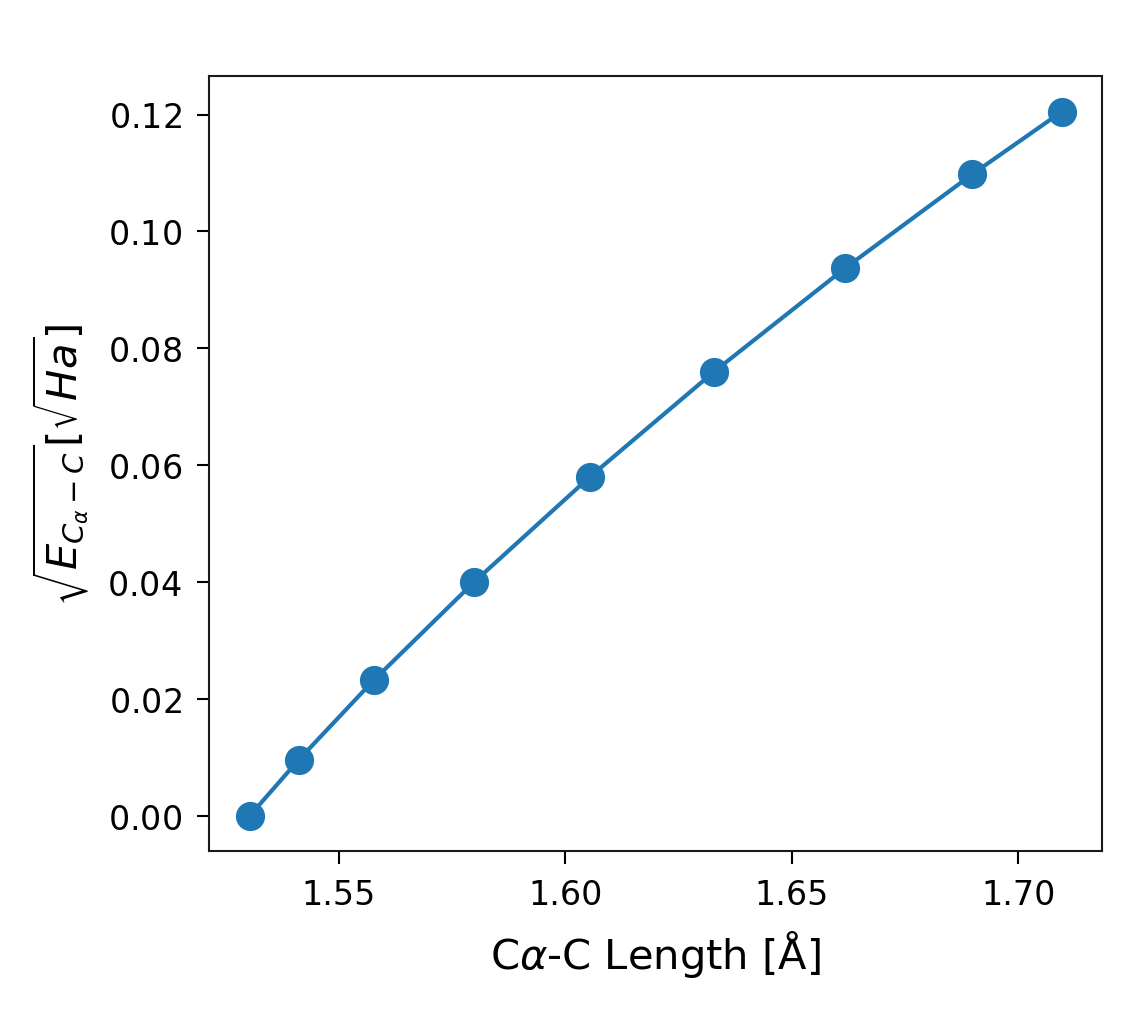
Figure 10. Square root of the energy stored in the degree of freedom corresponding to the distance between the C\(\alpha\) and C atoms of Glycine (second residue of the system).
Error Analysis in SITH
sith can also quantify the error relative to the total DFT energy change. Theory predicts that the sum of energy changes in all degrees of freedom equals the total molecular energy change. The following plot demonstrates that sith computes the energy distribution consistently with this expectation.
1plotter_sith.plot_error();
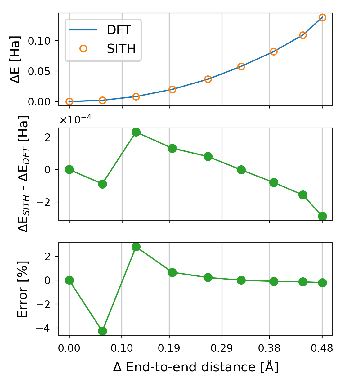
Figure 11. Different measurements of the error in sith. The reference value is the total DFT energy change.
Improved Representation of Angle Changes
Normal cartesian plots may not adequately display angle values due to their periodic
nature. We added the method
sith.utils.sith_plots.SithPlotter.plot_angles to
provide a clearer visualisation. The following plot shows the angle values:
1sp = plotter_sith.plot_angles(step=2)
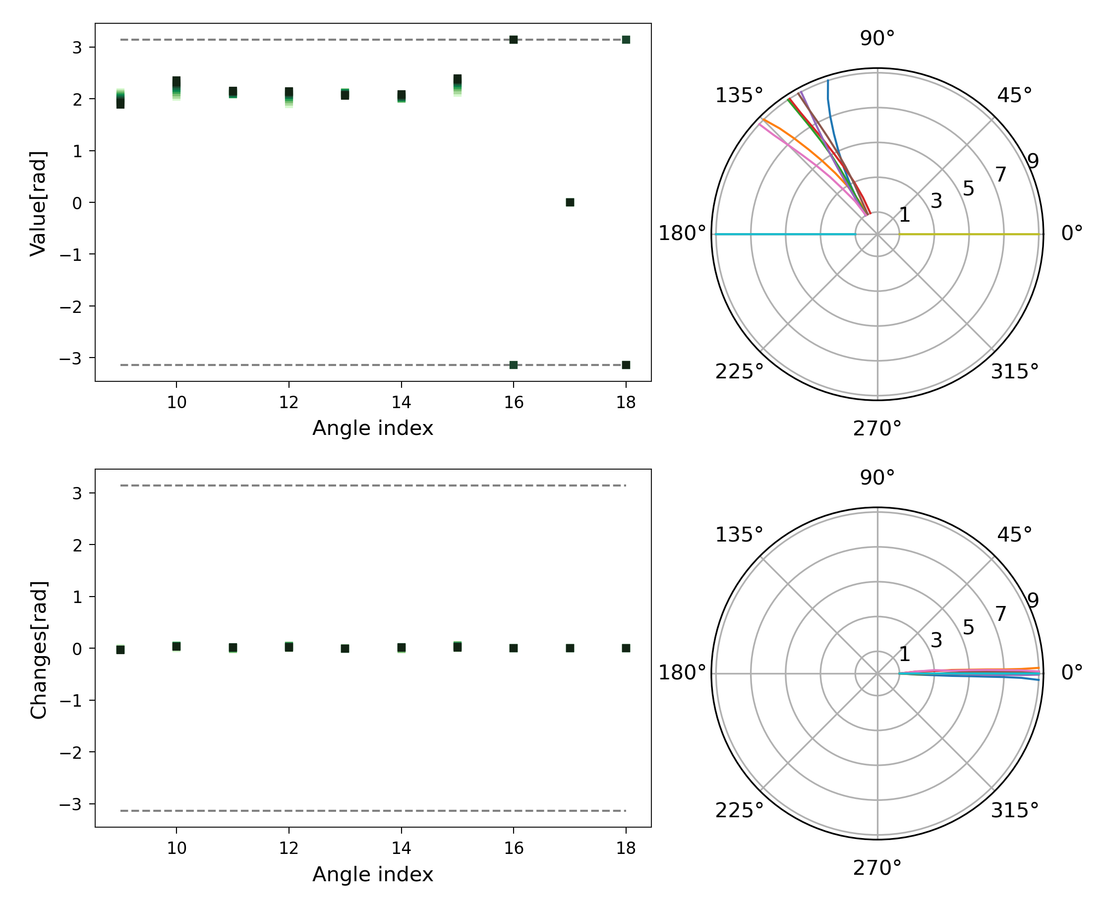
Figure 12. Representation of angles and their changes using a polar projection.