Beyond the candidates: machine learning
EPRoducer explains a spectrum only as well as its candidate radicals allow. Because a radical that the candidate set lacks cannot appear in the fit (see Linear combination of candidates), and every candidate costs a DFT optimization and a \(g\)-tensor calculation, the reconstruction of a spectrum depends on how well we anticipate its chemistry. We therefore propose a learning approach that derives the candidates from the spectrum itself and aims to explain any EPR spectrum.
Note
The models of this page are not part of EPRoducer. They are under development, and this page describes the approach and how it connects to EPRoducer.
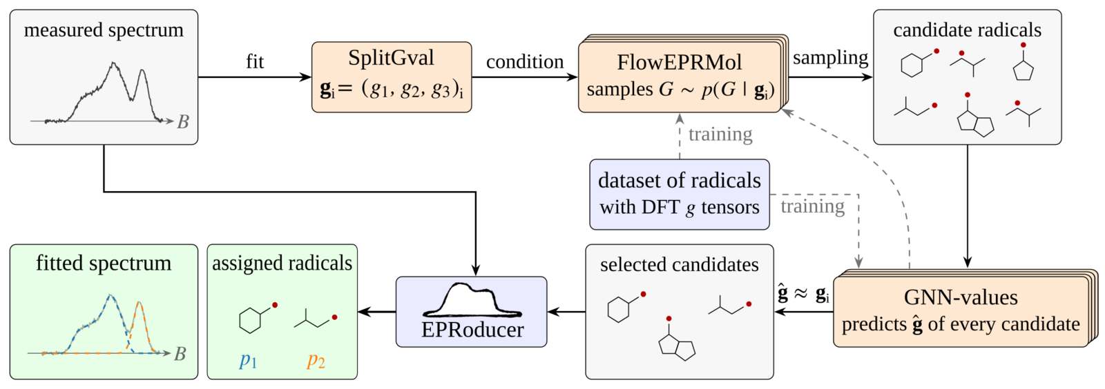
Learning radicals from EPR spectra. Orange blocks are machine learning models, blue blocks require quantum-chemical calculations, green blocks show the outcome, and grey blocks hold data. SplitGval splits the measured spectrum into effective \(g\) tensors \(\mathbf{g}_i\), one per radical species. For each \(\mathbf{g}_i\), FlowEPRMol samples candidate radicals \(G \sim p(G \mid \mathbf{g}_i)\), and GNN-values predicts the \(g\) tensor \(\hat{\mathbf{g}}\) of every candidate and keeps those with \(\hat{\mathbf{g}} \approx \mathbf{g}_i\). EPRoducer computes the \(g\) tensors of the selected candidates with DFT and fits the measured spectrum with their simulated spectra, which yields the assigned radicals, their proportions \(p_k\) and the fitted spectrum. Both models learn from a dataset of radicals with DFT \(g\) tensors, and GNN-values also guides the training of FlowEPRMol (dashed arrows).
The approach combines three machine learning models:
SplitGval splits the measured spectrum into a few effective \(g\) tensors \(\mathbf{g}_i = (g_1, g_2, g_3)_i\), one for each radical species that contributes to it.
FlowEPRMol takes one of these \(g\) tensors and generates radicals that have it, i.e. it samples radical structures \(G\) from the conditional distribution \(p(G \mid \mathbf{g}_i)\).
GNN-values takes a radical and predicts its \(g\) tensor \(\hat{\mathbf{g}}\) without a quantum-chemical calculation, which lets us discard the generated candidates whose \(\hat{\mathbf{g}}\) lies far from \(\mathbf{g}_i\).
The candidates that survive this screening enter EPRoducer, which computes their \(g\) tensors with DFT and fits the measured spectrum with them.
SplitGval
SplitGval is the simplest part of the workflow, although it has not been built yet. A suitable design can follow a simplified version of the representation of Xiong et al., who condition a generative model of molecules on one-dimensional NMR spectra [Xiong2025]. They interpolate each spectrum onto a fixed grid, normalize it to its highest peak, cut it into tokens with two one-dimensional convolutional layers, and process the tokens with a transformer encoder, whose attention relates separated peaks. For SplitGval, the grid can run over \(g\) instead of the magnetic field, so that spectra recorded at different microwave frequencies share one input format. The training spectra need no measurement or DFT data, because they can come from random combinations of parameters, random linear combinations and random noise, which reproduce experimental samples synthetically.
GNN-values
GNN-values is built on MACE, a message-passing neural network that learns atomic properties from the three-dimensional structure of a molecule [Batatia2022]. MACE represents a molecule as a graph in which every atom is a node connected to the atoms within a cutoff distance, and builds equivariant messages of high body order at a low cost, so that two or three layers already capture many-body correlations. Its readout uses only the invariant features.
GNN-values keeps this architecture and changes only what the readout predicts. Instead of one site energy, every layer reads out three invariant numbers per atom. GNN-values sums them over the layers and averages them over all atoms of the radical, which yields three numbers \((u_1, u_2, u_3)\) per radical. A monotonic parametrization turns them into the principal values,
where three constants of the training set fix the scale: the shift \(g_0 = 2.00198\) (mean of the smallest principal value), the scale \(s = 4.50\times10^{-3}\) (standard deviation of all principal values), and \(s_\Delta = 1.77\times10^{-3}\) (mean gap between neighbouring principal values). Because the softplus function \(\ln(1 + e^{u})\) is always positive, the prediction satisfies \(\hat{g}_1 \geq \hat{g}_2 \geq \hat{g}_3\) by construction. The loss is the squared error of the three principal values in units of \(s\),
averaged over the radicals of a batch, where \(g_k\) are the DFT values. Without the scaling, the deviations of about \(10^{-3}\) would produce gradients too small for the optimizer to act on. Averaging over all atoms frees GNN-values from knowing which atom hosts the unpaired electron, a label that the radicals generated by FlowEPRMol do not carry.
GNN-values is not trained from scratch. It starts from the foundation model MACE-OMOL-0 [Batatia2024], trained on four million structures of OMol25 [Levine2026], which also embeds the total charge and the spin multiplicity of the molecule. GNN-values inherits all its weights except those of the readout, and it is fine-tuned in two stages: first with a frozen backbone, so that the large gradients of the untrained readout cannot erase the pretrained features, and then with all parameters and a learning rate three orders of magnitude smaller.
Flow matching and FlowMol
Flow matching learns a time-dependent vector field that transports samples of a simple prior distribution \(p_0\) into samples of the data distribution \(p_1\) [Lipman2023]. Given a prior sample \(\mathbf{x}_0\) and a data sample \(\mathbf{x}_1\), the linear interpolant \(\mathbf{x}_t = (1-t)\,\mathbf{x}_0 + t\,\mathbf{x}_1\) defines a straight path whose velocity a neural network \(\mathbf{v}_\theta(\mathbf{x}_t, t)\) learns by regression,
Generation then integrates \(\mathrm{d}\mathbf{x}/\mathrm{d}t = \mathbf{v}_\theta(\mathbf{x}, t)\) from a prior sample at \(t = 0\) to \(t = 1\).
FlowMol extends flow matching to molecules \(G = (\mathbf{x}, a, c, e)\), which mix continuous atomic positions \(\mathbf{x}\) with categorical atom types \(a\), formal charges \(c\) and bond orders \(e\) [Dunn2024a] [Dunn2024b] [Dunn2025]. The positions follow the interpolant above, while the categorical variables follow discrete flow matching, in which a continuous-time Markov chain moves each variable out of a mask state [Campbell2024]. One network, built from geometric vector perceptrons [Jing2021], predicts the final molecule \(\hat{G}_1\) from the intermediate one \(G_t\), and the total loss is the weighted sum of the losses of the four modalities,
A “no bond” category and fake atoms leave the size and the connectivity of the generated molecule open.
FlowEPRMol
FlowEPRMol turns FlowMol into a conditional generative model that samples radicals for prescribed \(g\) values \(\mathbf{g} = (g_1, g_2, g_3)\), i.e. from \(p(G \mid \mathbf{g})\) rather than from \(p(G)\). The \(g\) values enter the model in two ways:
As context. The three principal values enter every atom as constant scalars, each through its own linear layer, and join the embeddings of the atom type, the formal charge and the time. Unlike the other variables, they do not follow a flow. At sampling time, every atom receives the target \(g\) values.
As a target. Similar to the flexibility loss with which Viliuga et al. generate protein backbones with a prescribed flexibility [Viliuga2025], GNN-values predicts the \(g\) values of the final molecule that the network predicts from \(G_t\), and an additional loss term compares them with the \(g\) values of the training radical,
(5)\[\mathcal{L}_{\mathbf{g}} = \mathrm{E}_{t,\,G_0,\,(G_1,\mathbf{g})} \left[ \frac{1}{3} \left\| \frac{\hat{\mathbf{g}}\big(\hat{G}_1(G_t, t, \mathbf{g})\big) - \mathbf{g}}{s} \right\|^2 \right] , \qquad \mathcal{L}_{\mathrm{FlowEPRMol}} = \mathcal{L}_{\mathrm{FlowMol}} + \lambda_{\mathbf{g}} \mathcal{L}_{\mathbf{g}} .\]
GNN-values stays frozen during this training, and it is made differentiable with respect to the atom types by replacing its one-hot encoding of the elements with the probabilities that FlowEPRMol predicts for them. GNN-values can also steer the sampling, by correcting the velocity of the positions with the gradient of the deviation from the target,
and rank its results with the standardized distance
Only the radicals with the smallest \(d\) proceed to the DFT calculations and the fit of EPRoducer.