Decomposing EPR spectra with EPRoducer

The usual interpretation of an EPR spectrum adjusts the parameters of the spin Hamiltonian, namely the \(g\) values, the hyperfine couplings and the line widths, by trial and error until a simulation matches the measurement. When several radicals share a powder spectrum, however, many parameter sets reproduce the same line shape. The fitted numbers alone then do not reveal which structures carry the unpaired electrons.

EPRoducer reverses the procedure. It proposes candidate radicals, computes their EPR parameters from first principles with ORCA (EPR parameters from first principles), simulates their spectra with EasySpin (Numerical EPR spectra), and searches for the combination of candidates that reproduces the measurement. Given that the fit then varies only the weight of each candidate, every parameter of the spin Hamiltonian keeps a structural origin.

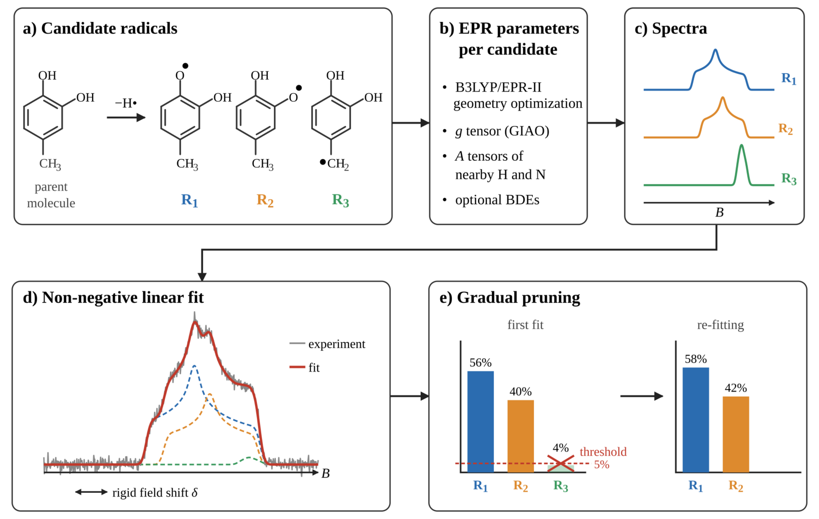
../_images/eproducer_workflow.png — Workflow of EPRoducer. a) Each candidate radical results from removing one hydrogen atom from a reference molecule, here a model of the DOPA side chain that yields two phenoxyl radicals (R₁, R₂) and one benzylic radical (R₃). b) ORCA computes the EPR parameters of every candidate. It optimizes the geometry with B3LYP/EPR-II and computes the \(g\) tensor with GIAOs, the hyperfine tensors of nearby H and N nuclei and, optionally, the BDEs with M06-2X. c) EasySpin simulates the solid-state powder spectrum of every candidate from these parameters. d) A non-negative linear combination of the simulated spectra, together with a rigid field shift \(\delta\), fits the experimental spectrum (grey), and the dashed curves show the weighted contribution of each candidate. e) A gradual pruning removes the candidates whose share \(p_k\) falls below a threshold, here 5%, and refits the remaining ones. The spectra and weights are illustrative.

The tutorial goes through these steps with a real example. The sections below explain what happens in each of them.

Candidate radicals and their EPR parameters

Each candidate encodes one hypothesis about where the unpaired electron sits. We start from a closed-shell parent molecule that represents the chemistry expected in the sample, such as a fragment of a crosslink (panel a), optimize it, and remove the hydrogen atoms whose abstraction would create the radicals of interest. A further deprotonation can change the total charge and, with it, the distribution of charge and spin over the atoms around the radical centre. Every candidate therefore carries its own charge and a doublet multiplicity, and the subsequent calculations treat it as an independent molecule.

EPRoducer computes the EPR parameters of every candidate with ORCA [Neese2022] (panel b):

Optimization. Each candidate is optimized with the B3LYP functional and the EPR-II basis set, which is replaced by def2-TZVP for P, S, Cl and Br, since EPR-II does not cover them.
g tensor. At the optimized geometry, the same level of theory yields the \(\mathbf{g}\) tensor, with gauge-including atomic orbitals that remove the dependence on the gauge origin [Ditchfield1974] (see Gauge origin).
Hyperfine tensors. They cost more and, as explained in Simulated spectra, shape high-field spectra little. Their effect also decreases with the distance from the radical centre, so EPRoducer computes them only for selected nuclei. Starting from the atoms that may host the radical, it walks along the bonds up to a chosen number of connected neighbours and collects the atoms with relevant nuclear spin, i.e. the hydrogens (\(I=1/2\)) and nitrogens (\(I=1\)) of organic molecules.
Enthalpies (optional). A re-optimization and frequency calculation at the M06-2X/def2-TZVP level provides the enthalpies that the bond dissociation enthalpies (BDEs) require. BDEs can be used as an additional stability measure of the candidates.

In EPRoducer

gval_workflow runs these steps for one candidate (gval_dataset for many radicals of an npz dataset):

-c and -m: charge and multiplicity (2 by default).
-x: functional and basis set of the EPR calculation (B3LYP EPR-II by default).
-f: atoms included in the hyperfine calculation. An argument that starts with g guesses them with eproducer.g_valsetup.HFC_relevantA(), which collects the H, O and N atoms (and the H atoms bonded to O and N) within d bonds of the given atoms, e.g. 'g1,4d2'.
-g/-r: guess the radical centre by comparison with the molecule before the hydrogen abstraction (see eproducer.g_valsetup.rad_loc()).
-b: skip the M06-2X frequency calculation; -e: skip the EPR calculation (e.g. to optimize the closed-shell parent molecule).

Bond dissociation enthalpies

For a homolytic cleavage \(\mathrm{A}\text{-}\mathrm{B} \rightarrow \mathrm{A}^{\bullet} + \mathrm{B}^{\bullet}\) of a bond \(i\), the BDE is the enthalpy required to cleave that bond,

(1)\[D_i = H(\mathrm{A}^{\bullet}) + H(\mathrm{B}^{\bullet}) - H(\mathrm{A}\text{-}\mathrm{B}) ,\]

with every species relaxed to its own minimum and zero-point vibrational energies included. Two bonds of the same type in different molecular environments generally have different \(D_i\). For hydrogen abstractions, the isolated H atom is a one-electron system that exposes the self-interaction error of DFT functionals. The isodesmic variant [Hehre1970] [Chan2021] replaces \(H(\mathrm{H}^{\bullet})\) by the experimental BDE of a reference molecule \(\mathrm{Y}\text{-}\mathrm{H}\) that resembles the molecule of interest \(\mathrm{X}\text{-}\mathrm{H}\),

(2)\[D_i^{\mathrm{iso}}(\mathrm{X}) = \left[H(\mathrm{X}^{\bullet}) - H(\mathrm{Y}^{\bullet})\right] + \left[H(\mathrm{Y}\text{-}\mathrm{H}) - H(\mathrm{X}\text{-}\mathrm{H})\right] + D^{\mathrm{exp}}(\mathrm{Y}) .\]

In EPRoducer

eproducer.postpro.compute_bde() returns the enthalpy of the products minus that of the reactants, read from the frequency outputs of ORCA:

# BDE of the bond A-B
eproducer compute_bde --reactants "['AB_freq.out']" --products "['A_freq.out', 'B_freq.out']"
# isodesmic BDE of X-H with the reference Y-H, without the term D_exp(Y)
eproducer compute_bde --reactants "['XH_freq.out', 'Y_freq.out']" --products "['X_freq.out', 'YH_freq.out']"

Simulated spectra

Once the calculations finish, EasySpin reads the ORCA output and simulates the powder spectrum of each candidate (panel c) with its solid-state routine [Stoll2006], using the microwave frequency and the field range of the experiment. The simulation yields the absorption spectrum by default, and it can also return a field derivative with a given modulation amplitude. All candidates share one peak-to-peak line width, 1 mT unless chosen otherwise.

By default, the simulation leaves out the hyperfine couplings and keeps only the \(\mathbf{g}\) tensor, because at high field the \(\mathbf{g}\) tensor dominates the spectrum, and the hyperfine correction is computationally expensive. A candidate with large couplings is the exception, for which the couplings of the selected nuclei are kept in the simulation.

In EPRoducer

extract_EPRspec simulates the spectrum of a candidate from its ORCA output (-f keeps the hyperfine couplings). See Line broadening and detection for the meaning of its flags.

Linear combination of candidates

EPRoducer fits the measured spectrum with a non-negative linear combination of the simulated candidate spectra (panel d). It normalizes the experimental intensity to its maximum, \(I_{\mathrm{exp}}(B_m)\) at the experimental field points \(B_m\), and interpolates the simulated spectrum \(S_k(B)\) of every candidate \(k\) onto those points. The fit then solves

(3)\[\min_{\delta}\ \min_{c_k \geq 0}\ \sum_m \left[ I_{\mathrm{exp}}(B_m) - \sum_k c_k\, S_k(B_m + \delta) \right]^2 ,\]

where \(c_k\) weighs candidate \(k\) and \(\delta\) shifts the field axis rigidly.

For every \(\delta\), a non-negative least-squares algorithm solves the inner minimization exactly, while the outer one scans \(\delta\) on a regular grid within a symmetric window and keeps the value with the smallest residual.
The non-negativity reflects the physics, since a radical cannot contribute a negative absorption. It also sets the weight of every candidate that does not improve the fit to exactly zero.
The shift absorbs small offsets in the field and microwave frequency calibration and, since a uniform field shift acts approximately like a uniform change of all \(g\) values, also a systematic error of the computed \(g\) values that all candidates share.
An optional field window confines the comparison to the region where the candidates should contribute, because the fit takes the experimental intensity outside that window as zero. This window helps when only one part of the spectrum is meant to be simulated, avoiding, for example, fitting a part of the spectrum produced by impurities in the sample.

Gradual pruning

A gradual pruning keeps only the candidates that matter (panel e). It relies on the normalized weights

(4)\[p_k = 100\,\frac{c_k}{\sum_j c_j} ,\]

which give the percentage that each candidate contributes to the fitted spectrum. The pruning raises a threshold on \(p_k\) step by step (for example from 1% to 5% in steps of 1%), discarding at each step the candidates below it and fitting again. The gradual removal lets the weights redistribute after every step, instead of discarding at once a candidate that would gain weight once its weaker competitors leave. In the final combination, every candidate contributes at least the final threshold. Because all simulated spectra refer to the same number of spins, \(p_k\) estimates the share of radical \(k\) among the paramagnetic species of the sample. This pruning avoids overfitting and minimizes the number of chemical moieties that explain an EPR spectrum.

In EPRoducer

From the terminal,

eproducer best_fit <experiment.dat> <fit.png> '[min, max]' <candidate1.dat> <candidate2.dat> ...

fits the experiment with the spectra of the candidates, prints the percentage \(p_k\) of each remaining candidate and the shift \(\delta\), and saves a plot of the fit (use '' instead of '[min, max]' to fit the whole field range). It scans \(\delta\) within \(\pm 10\) field units (mT for the spectra of EasySpin) in steps of 0.2, and raises the pruning threshold from 0.1% to 5% in steps of 0.1%.

From Python, eproducer.best_fit.TheoMatchExpe gives control over every setting:

fit_theoretical() solves the inner minimization of Eq. (3) for a fixed shift, with an optional field window (fieldrange).
fit_shifting() scans the shift (shifting_width, shift_step).
proportions() computes the percentages of Eq. (4).
gradual_cleaning() runs the gradual pruning (threshold, steps).

Besides the residual of the fit, EPRoducer reports the Pearson correlation between the fitted and the experimental spectra. The fitting tutorial shows how the shift and the field range improve a fit and why both measures are reported.

Limitations

The main limitation of the method is that it can only find what the set of candidates contains. A radical that is not among the candidates cannot appear in the fit, and choosing the candidates relies on chemical intuition and on prior knowledge of the sample. Beyond the candidates: machine learning proposes an alternative to overcome this problem.