Quantifying the quality of a Fitting
Importing packages
[1]:
from eproducer.best_fit import TheoMatchExpe
from PlottingTool import StandardPlotter
from scipy.stats import pearsonr
import numpy as np
Best fitting of a function as a linear combination of another
We take two functions, f(x) and g(x) = f(x + 8). We try to automatically find a coefficient c, such that c * g(x) minimizes the error with respect to f(x).
[2]:
tme = TheoMatchExpe(['shifted-spectrum2.dat'],
                    experiment_file='spectrum2.dat')

sp = StandardPlotter(ax_pref={'xlabel': 'Field [T]',
                              'ylabel': 'Intensity [a.u]'},
                     plot_pref={'pstyle': '-'})

sp.plot_data(tme.fieldexp, tme.intensexp, pstyle='-', color_plot='black', data_label='Experiment')
sp.plot_data(tme.fieldexp, tme.coeffs[0] * tme.intensities[0], pstyle='--', data_label="'expected'");
#sp.plot_data([limi[0], limi[0]], [0,1], pstyle='--', color_plot='black');
#sp.plot_data([limi[1], limi[1]], [0,1], pstyle='--', color_plot='black');
sp.axis_setter(legend=True)
[2]:
<Axes: xlabel='Field [T]', ylabel='Intensity [a.u]'>
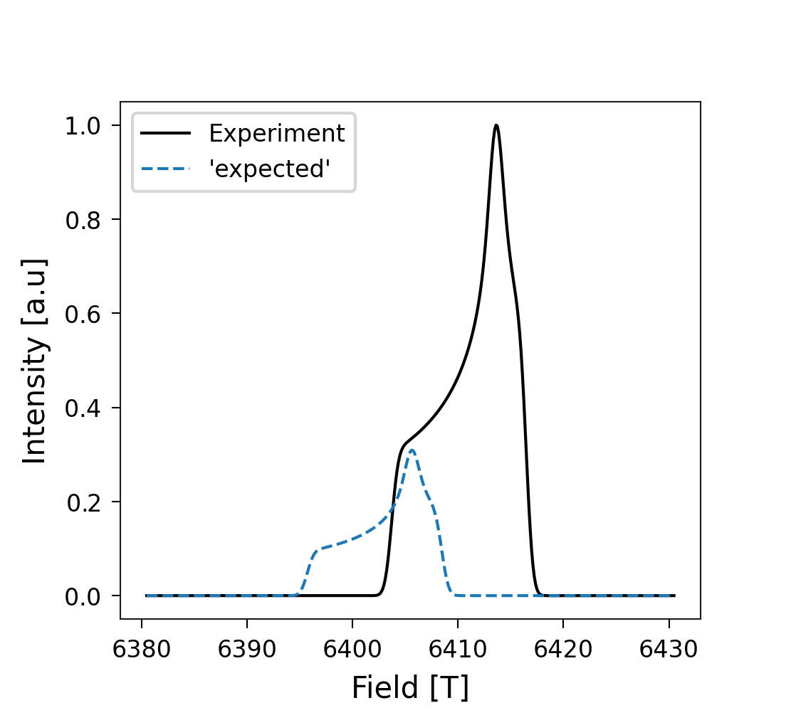
In this case, tme.coeffs[0] is the expected c, and the correlation and error are:
[3]:
tme.corr, tme.error
[3]:
(np.float64(0.10279243360690807), 5.4180832414280315)
Now assume that we don’t know the value d that maximizes the fit of g(x + d) to f(x). By definition, it is 8 (in absolute value), but let’s find it automatically.
[4]:
tme = TheoMatchExpe(['shifted-spectrum2.dat'],
                    experiment_file='spectrum2.dat',

                     shifting_width=10)

sp = StandardPlotter(ax_pref={'xlabel': 'Field [T]',
                              'ylabel': 'Intensity [a.u]'}
                     )

sp.plot_data(tme.fieldexp, tme.intensexp, pstyle='-', color_plot='black', data_label='Experiment')
sp.plot_data(tme.fieldexp, tme.coeffs[0] * tme.intensities[0], pstyle='--', data_label="'expected'");
sp.axis_setter(legend=True)
[4]:
<Axes: xlabel='Field [T]', ylabel='Intensity [a.u]'>
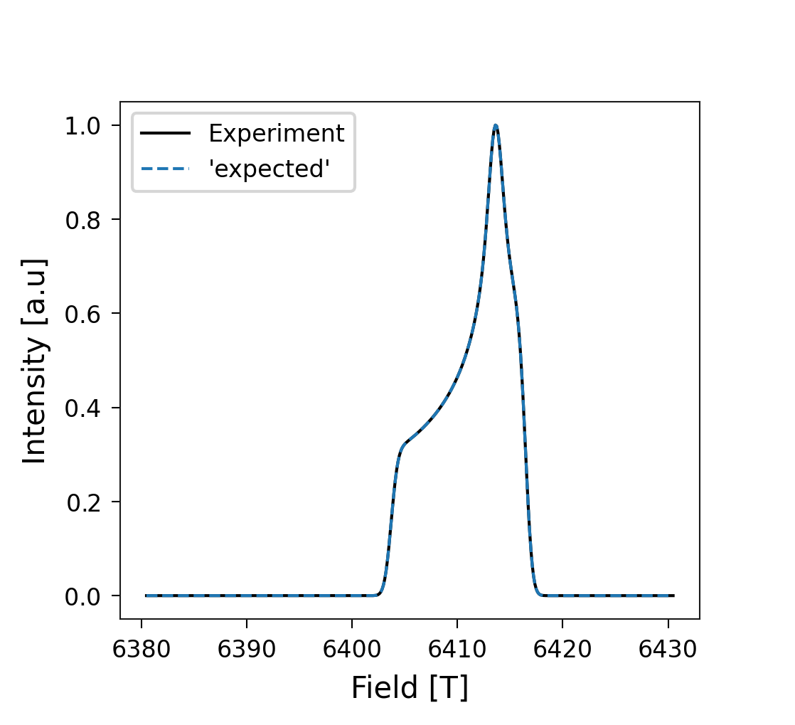
We can see that the predicted shift is as expected:
[5]:
tme.shift
[5]:
np.float64(-8.000000000000007)
And with this trick, the correlation improved:
[6]:
tme.corr, tme.error
[6]:
(np.float64(1.0), 1.895521140103284e-15)
Fitting a function that matches only part of another
Now let’s take a function g(x) which fits another function f(x) only in a range a < x < b. If we fit the whole spectrum, the fit is quite bad:
[7]:
tme = TheoMatchExpe(['spectrum2.dat'],
                    experiment_file='spectrum1.dat',

                     shifting_width=0)

sp = StandardPlotter(ax_pref={'xlabel': 'Field [T]',
                              'ylabel': 'Intensity [a.u]'})

sp.plot_data(tme.fieldexp, tme.intensexp, pstyle='-', color_plot='black', data_label='Experiment')
sp.plot_data(tme.fieldexp, tme.coeffs[0] * tme.intensities[0], pstyle='--', data_label="'expected'");
sp.axis_setter(legend=True)
[7]:
<Axes: xlabel='Field [T]', ylabel='Intensity [a.u]'>
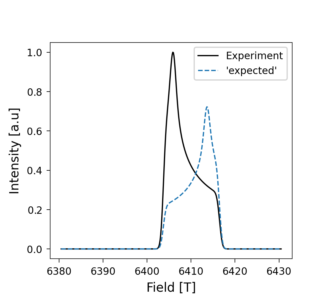
In this case, tme.coeffs[0] is the expected c, and the correlation and error are:
[8]:
tme.corr, tme.error
[8]:
(np.float64(0.6826351345562202), 3.5777191120542136)
Even using the translation trick, the fit doesn’t work so well:
[9]:
tme = TheoMatchExpe(['spectrum2.dat'],
                    experiment_file='spectrum1.dat',

                     shifting_width=10)

sp = StandardPlotter(ax_pref={'xlabel': 'Field [T]',
                              'ylabel': 'Intensity [a.u]'})

sp.plot_data(tme.fieldexp, tme.intensexp, pstyle='-', color_plot='black', data_label='Experiment')
sp.plot_data(tme.fieldexp, tme.coeffs[0] * tme.intensities[0], pstyle='--', data_label="'expected'");
sp.axis_setter(legend=True)
[9]:
<Axes: xlabel='Field [T]', ylabel='Intensity [a.u]'>
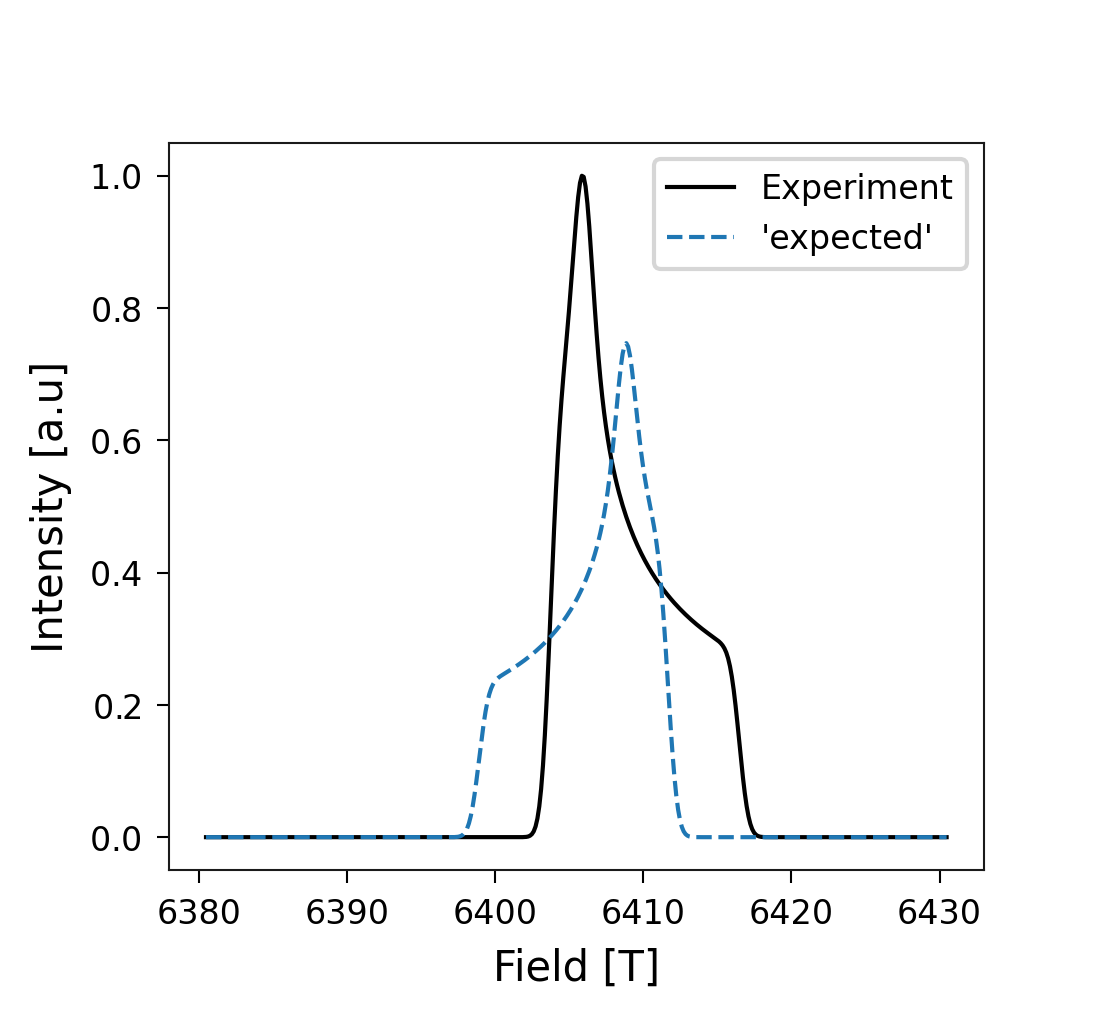
The correlation improves, but only slightly:
[10]:
tme.corr, tme.error
[10]:
(np.float64(0.7165595748192071), 3.4061899143036474)
[11]:
limi = [6404, 6407.5]

tme = TheoMatchExpe(['spectrum2.dat'],
                    experiment_file='spectrum1.dat',
                    fieldrange=limi,
                     shifting_width=10)

sp = StandardPlotter(ax_pref={'xlabel': 'Field [T]',
                              'ylabel': 'Intensity [a.u]'})

sp.plot_data(tme.fieldexp, tme.intensexp, pstyle='-', color_plot='black', data_label='Experiment')
sp.plot_data(tme.fieldexp, tme.coeffs[0] * tme.intensities[0], pstyle='--', data_label="'expected'");
sp.plot_data([limi[0], limi[0]], [0,1], pstyle='--', color_plot='gray');
sp.plot_data([limi[1], limi[1]], [0,1], pstyle='--', color_plot='gray');
sp.axis_setter(legend=True)
[11]:
<Axes: xlabel='Field [T]', ylabel='Intensity [a.u]'>
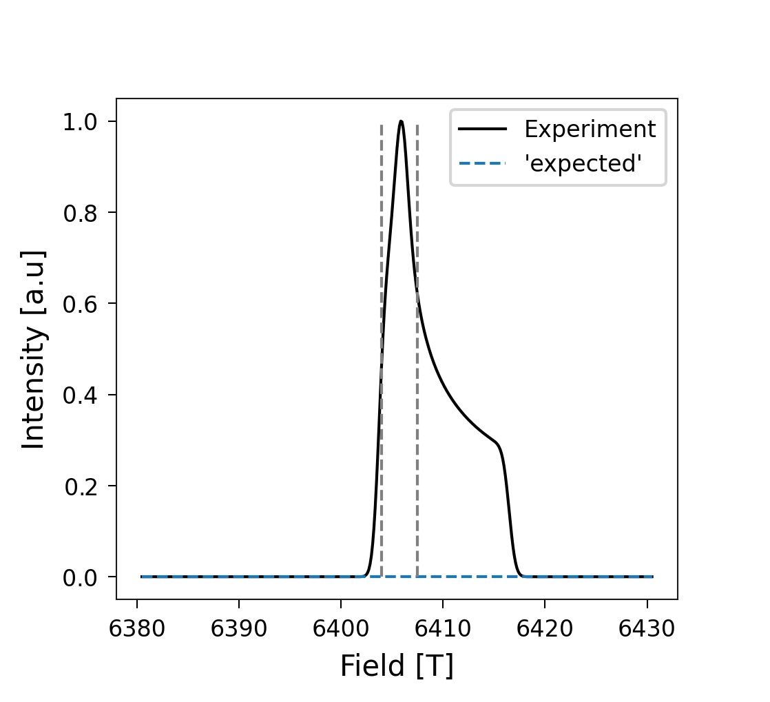
[12]:
tme.corr, tme.error
[12]:
(np.float64(0.7002899241650604), 3.441514309504788e-16)
Inside fieldrange the fit is now almost perfect: the error is computed with the experiment set to zero outside that range, so it drops to ~0. The correlation, in contrast, is computed with the whole experimental spectrum, which includes the parts that spectrum2.dat does not describe.
Why error and correlation?
In certain applications, we need a quantity that says which function fits better independent of the scale and the translation in the y axis. Let’s see what happens with the error and the correlation when we compare f(x) vs g(x) with f(x) vs a * g(x) + b
[13]:
tme = TheoMatchExpe(['shifted-spectrum2.dat'], experiment_file='spectrum2.dat')
[14]:
error = np.linalg.norm(tme.intensexp - tme.intensfit)
corr = pearsonr(tme.intensexp, tme.intensfit)[0]

print(f'error of f(x) vs g(x): {error:0.5f}')
print(f'correlation of f(x) vs g(x): {corr:0.5f}')
error of f(x) vs g(x): 5.41808
correlation of f(x) vs g(x): 0.10279
[15]:
error = np.linalg.norm(tme.intensexp - 7 * tme.intensfit + 4)
corr = pearsonr(tme.intensexp, 7 * tme.intensfit + 4)[0]

print(f'error of f(x) vs g(x): {error:0.5f}')
print(f'correlation of f(x) vs 7*g(x)+4: {corr:0.5f}')
error of f(x) vs g(x): 77.76395
correlation of f(x) vs 7*g(x)+4: 0.10279
Notice that the correlation does not depend on the scale and translation on the y axis.