Theoretical EPR spectrum

Attention

To use the tools of EPRoducer that are part of this tutorial, be sure that ORCA, MATLAB (with EasySpin) and VMD are well set up. Check ORCA and MATLAB set up for more information.

For the impatient

This tutorial builds a whole project. If you only want to compute the g-values of a molecule with a radical that you already know, go directly to Compute the g-values.

Suppose that you have an EPR absorption spectrum that you got from a sample of collagen that looks like this:

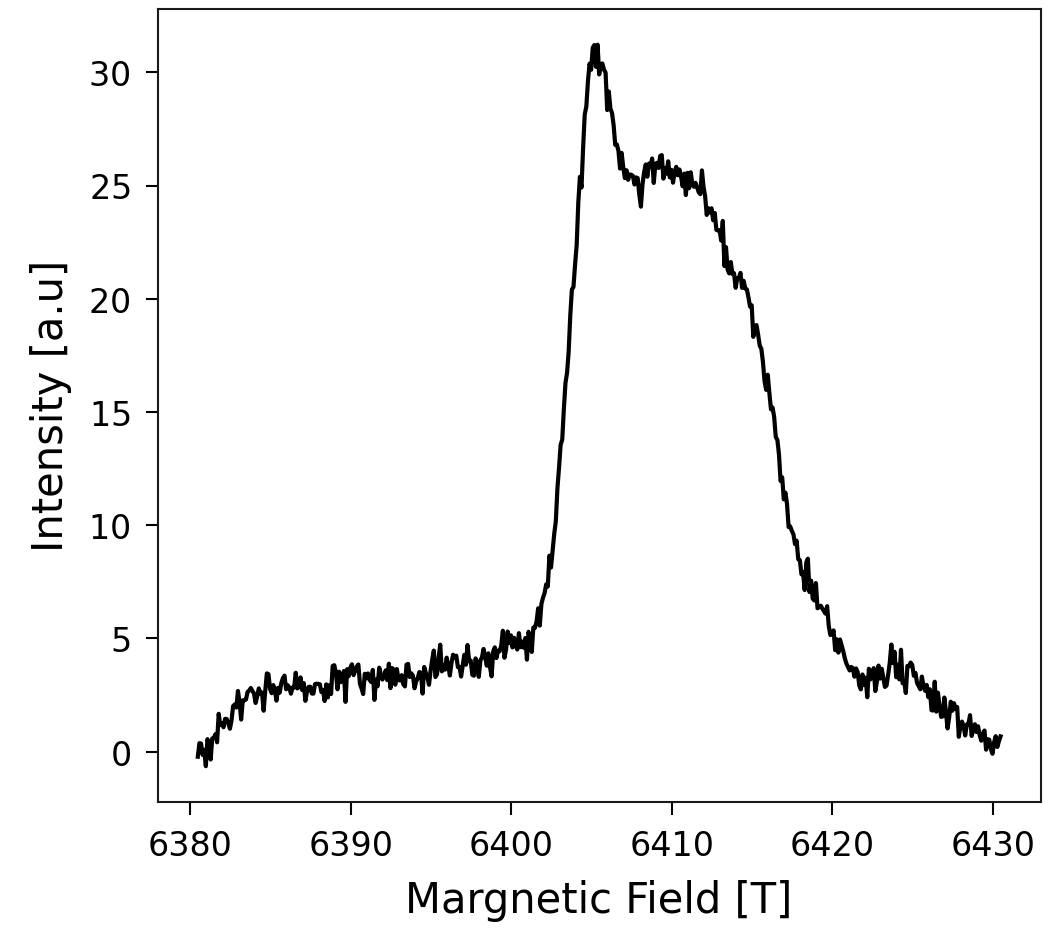
In this tutorial, you will learn how to discover which radical species this spectrum comes from, using EPRoducer. This process is usually done by finding, by trial-and-error, the g-values that best fit the experiment. Our procedure, in contrast, consists of computing the spectra of some candidates that you expect in your sample and finding which ones fit the spectrum. With the final fit, you obtain the concentration of each radical species in your sample. In this case, we are going to assume a rupture of trivalent crosslinks, which were shown to be sacrificial bonds by Rennekamp, et al., 2023.

System

Consider the radicals in a broken trivalent crosslink, which corresponds to the following molecule:

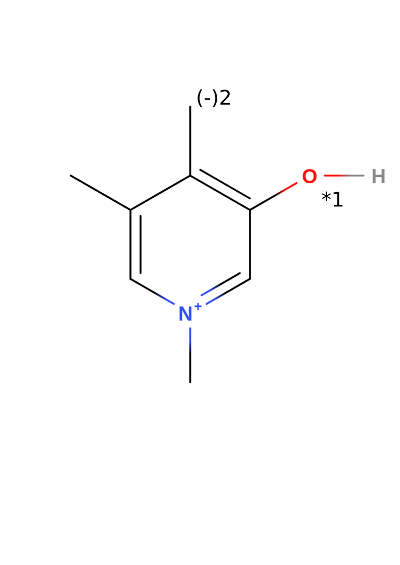
Note that the structure of this example without radicals has a total charge of +1. The numbers 1 and 2 in the image represent the two candidates that we are going to consider in this tutorial. Candidate 1 results from taking out the hydrogen bonded to the oxygen and increasing the multiplicity to 2 (radical). Candidate 2 results from deprotonating the methyl group of the first candidate, which leads to a total charge of zero. Since the DFT calculation determines how the charges are distributed, the second candidate can also be seen as a radical in the methyl group and a negative charge in the oxygen.

Starting a new project

To use all the advantages of EPRoducer, the files must follow a specific folder structure, which you will build step by step during this tutorial. The general structure looks like this:

<project>/
├── experiments/
└── <molecule>/
    ├── opt/
    └── <i>-<radical name>/

Here, “<project>” is the name of the whole project, “<molecule>” is the molecule that you use as a base to create the radical candidates, and “<i>-<radical name>” is the directory of the i-th radical candidate, where “<i>” is a number and “<radical name>” a name of your choice. For this tutorial, the tree looks like this:

CollagenEPR/
├── experiments/
└── PYD/
    ├── opt/
    ├── 1-OxygenCharged/
    └── 2-OxygenNeutral/

Your task now is to create this folder structure:

mkdir CollagenEPR
mkdir CollagenEPR/experiments
mkdir CollagenEPR/PYD
mkdir CollagenEPR/PYD/opt
mkdir CollagenEPR/PYD/1-OxygenCharged
mkdir CollagenEPR/PYD/2-OxygenNeutral

Now save your absorption spectrum in the “experiments” directory as CollagenEPR/experiments/field_intensity.dat. You can save as many measurements as you have. They should be .dat files with two columns: field and intensity.

Create a model

To compute radicals, you need an XYZ file with the molecular coordinates. You can build it with your favorite tool. We recommend https://molview.org, which allows you to build your molecule from the structural formula and download its coordinates.

Note

To transform the .mol file downloaded from MolView into an .xyz file, use

obabel model.mol -O CollagenEPR/PYD/opt/model.xyz

You might want to save an image of your molecular structure, because at the end we are going to summarize the results in a clear and easy way. That image should also show the labels of the candidates, as in the image above. Save it as CollagenEPR/PYD/molecule.png.

Optimize the model

Depending on how you built your molecule, the model could be far from a stable configuration. Be aware that the g-values of the candidates have to be computed with optimized configurations. Optimizing the initial model can speed up the subsequent optimizations of the radicals derived from it, which pays off when you have several candidates. It is optional, though, because each radical is optimized again when its g-values are computed. If you already have a good structure, or if you want to skip this step, copy your model to

cp CollagenEPR/PYD/opt/model.xyz CollagenEPR/PYD/opt/model_opt.xyz

and continue to the next section. Otherwise, optimize your structure with EPRoducer:

cd CollagenEPR/PYD/opt
$(eproducer gval_workflow -path) -c 1 -m 1 -e -v

The flag -e skips the computation of the g-values and the hyperfine couplings (HFC), which would not make sense here because this molecule has no radical. The optimized structure is saved in model_opt.xyz. Use eproducer gval_workflow -h to check the role of the other flags.

Note

gval_workflow is a bash script with #SBATCH options for the SLURM queue system, so you can also submit it to an HPC cluster with sbatch $(eproducer gval_workflow -path) .... To modify those options or add the ones of your queue system, make a copy of the script with cp $(eproducer gval_workflow -path) ./<name_of_preference>.sh and submit your copy. You can also use it to understand and modify this code according to your style. If you improve the project, don’t hesitate to contribute your changes to EPRoducer.

Create radical models

Use the optimized model to create the radical candidates. You can do that by removing the hydrogen atom that caps each radical site. One way to do that is viewing your molecule with your favorite visualization tool (VMol, PyMol, VMD…) to check the index of the atom and remove it. Save the xyz file of each modified molecule in a new directory called <i>-<radical name>. In this case, we create the radical candidates from CollagenEPR/PYD/opt/model_opt.xyz: candidate 1 is obtained by removing the hydrogen 6, and candidate 2 by removing the hydrogens 6 and 16 (indices starting from 1). Considering that the xyz format includes two heading lines (a first line with the number of atoms and a second line for comments), the 6th and 16th atoms correspond to the 8th and 18th lines, respectively. Then, from the folder “CollagenEPR/PYD”, we execute the following commands to remove those atoms from the optimized molecule and save the outcome in the proper directory:

sed -E "1s/.*/21/ ; 8d" opt/model_opt.xyz > 1-OxygenCharged/model.xyz
sed -E "1s/.*/20/ ; 18d ; 8d" opt/model_opt.xyz > 2-OxygenNeutral/model.xyz

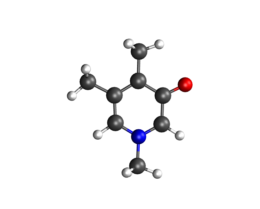
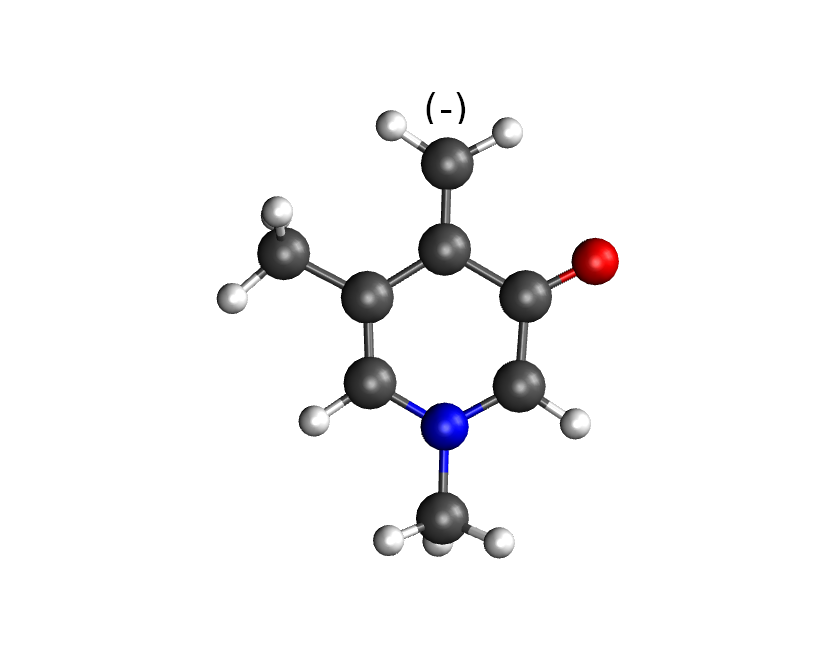
The resulting molecules should look like the following figure (candidate 1 on the left, candidate 2 on the right):

Compute the g-values

Once you have the file <i>-<radical name>/model.xyz of each radical, run

cd 1-OxygenCharged
$(eproducer gval_workflow -path) -c 1 -f 'g1,4d2' -v
cd ../2-OxygenNeutral
$(eproducer gval_workflow -path) -c 0 -f 'g1,4,6d2' -v

The flag -f indicates which atoms should be included in the hyperfine calculation. If its argument starts with g, eproducer.g_valsetup.HFC_relevantA() is used to guess the H, O and N atoms around the possible radical locations. For example, 'g1,4d2' means: guess (g) the relevant atoms around the atoms 1 and 4, up to two bonds away (d2). The indices start from 1 and refer to the model.xyz file of each candidate, so they can differ from the indices in the original molecule because some hydrogens were removed. In this case, for the HFC, we included all the atoms selected by HFC_relevantA around the nitrogen (index 1), the oxygen (index 4) and, in candidate 2, the carbon that can be charged (index 6). For more information about the guess function and the other flags, use eproducer gval_workflow -h. This workflow does what is explained in the ORCA tutorial and in Zhe Wang’s tutorial. In each candidate directory, it creates model_opt.xyz (optimized radical), model_epr.out (g-values and HFC) and model_freq.out (frequencies).

Note

gval_workflow is a bash script that you can modify. See last comment for more details.

Tip

gval_workflow also computes frequencies by default, which includes the computation of thermal properties. In particular, it computes the enthalpy of the molecule, which is useful to compute bond dissociation enthalpies (BDEs). If you want to skip this part, use the flag -b.

Compute the spectra

With the g-values and the hyperfine couplings, compute the theoretical spectrum of each candidate with EasySpin, using the field range of your experiment:

cd 1-OxygenCharged
$(eproducer extract_EPRspec -path) -e ../../experiments/field_intensity.dat -O model_epr.out -f
cd ../2-OxygenNeutral
$(eproducer extract_EPRspec -path) -e ../../experiments/field_intensity.dat -O model_epr.out -f

The flag -f includes the hyperfine corrections, which requires a lot of memory. The spectrum is saved in spectrum_wo_hyFiCorr.dat, the file that the next steps look for. Despite its name (“without hyperfine correction”), the file keeps this name also with -f. The default microwave frequency (179.813 GHz) corresponds to G-band experiments; use the flag -m for other bands. Check eproducer extract_EPRspec -h for the other flags.

Postprocessing

Once your calculations are complete, you can use eproducer gval_postpro to:

• Render each model in a file called opt.png

• Plot the g-values of all the candidates in a file called gvalues.png

• Create a table of the g-values in gvalues_table.md

• Create a file called vmd_image.md in each one of the candidate directories, with the comparison of its spectrum with each experiment.

Move to the project folder (CollagenEPR) and run

$(eproducer gval_postpro -path) -c PYD/ -e ../../experiments/field_intensity.dat -O model_epr.out

The paths given with -e are relative to the candidate directories (PYD/<i>-<radical name>/), where the spectra are compared.

Summarize your results

With the information obtained from the postprocessing, you can write a proper README.md file to summarize your results. eproducer gvals_template makes this step quite easy. Copy the template to your project folder with cp $(eproducer gvals_template -path) ./write_readme.sh. This template creates the README. To adapt it to your own project, modify the blocks delimited by EOF with the corresponding information. Also, change the parts that have <replace:. Then, run it and redirect its output to README.md. In this case, we do

cp $(eproducer gvals_template -path) ./write_readme.sh
sed -i "s/<replace: name of your candidates>/PYD/g" write_readme.sh
sed -i "s/<replace: experiment>/field_intensity/g" write_readme.sh
sed -i "s/<replace: fitting name>/fit2exper1/g" write_readme.sh
./write_readme.sh > README.md

and this creates a markdown file with the summary of all the results. Render your project with your tool of preference. GitHub and GitLab render these files automatically. Your whole project should now look like the repository github.com/Sucerquia/collagenEPR.

Tip

You can transform your README.md into a webpage using GitHub Pages.

Fit

At the end of the summary, there is an image of the best possible fit with your candidates. In this case, it should look like this

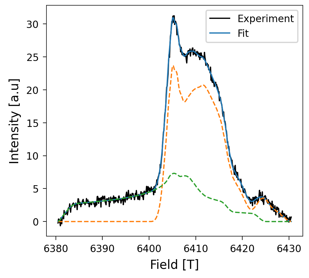
Great fit, isn’t it?! Now the question is how much of the spectrum comes from each candidate. The answer to this question is in the table at the end of the README. The outcome in this case is

System	Percentage (%)
PYD/2-OxygenNeutral	70.04
PYD/1-OxygenCharged	29.96

You got a perfect description of your EPR spectrum with the candidates you took into account! Now, you can use it with your own experimental data and radical candidates.